import numpy as np
import pandas as pd
import pandas_datareader.data as pdr
import matplotlib.pyplot as plt

import datetime

import torch
import torch.nn as nn
from torch.autograd import Variable

import torch.optim as optim
from torch.utils.data import Dataset, DataLoader
2️⃣ 삼성 전자 주식 불러오기
삼성전자의 종목코드는 005930
start = (2000, 1, 1) # 2020년 01년 01월
start = datetime.datetime(*start)
end = datetime.date.today() # 현재
# yahoo 에서 삼성 전자 불러오기
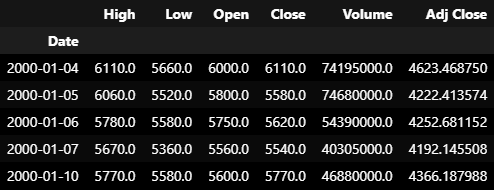
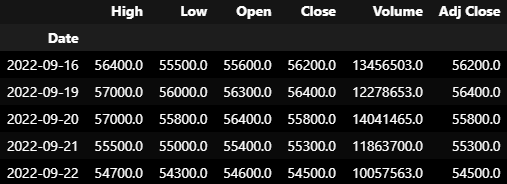
df = pdr.DataReader('005930.KS', 'yahoo', start, end)
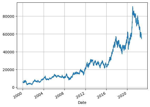
df.Close.plot(grid=True)
2022.09.22 기준으로 요즘 주식 장 파란불~이다 ㅠㅠㅠㅠ내림추세ㄴ
3️⃣ 모델 성능 학습하기위해 데이터 분류하기
open 시가
high 고가
low 저가
close 종가
volume 거래량 (필요 없어서 DROP)
Adj Close 주식의 분할, 배당, 배분 등을 고려해 조정한 종가 (예측하고자 하는 TARGET)
X = df.drop(columns='Volume')
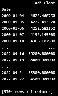
y = df.iloc[:, 5:6]
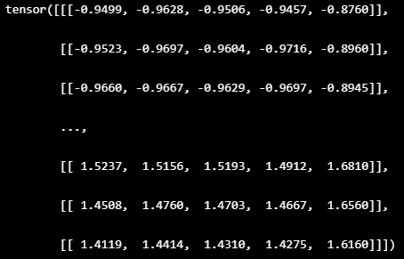
print(X)
print(y)
4️⃣ 학습이 잘되기 위해 데이터 정규화 및 split
StandardScaler : 각 특징의 평균을 0, 분산을 1이 되도록 변경
MinMaxScaler : 최대/최소값이 각각 1, 0이 되도록 변경
from sklearn.preprocessing import StandardScaler, MinMaxScaler
from sklearn.model_selection import train_test_split
mm = MinMaxScaler()
ss = StandardScaler()
X_ss = ss.fit_transform(X)
y_mm = mm.fit_transform(y)
X_train, X_test, y_train, y_test = train_test_split(X_ss, y_mm, test_size=0.2, shuffle=True, random_state=34)
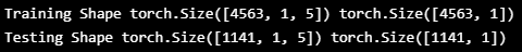
print("Training Shape", X_train.shape, y_train.shape)
print("Testing Shape", X_test.shape, y_test.shape)
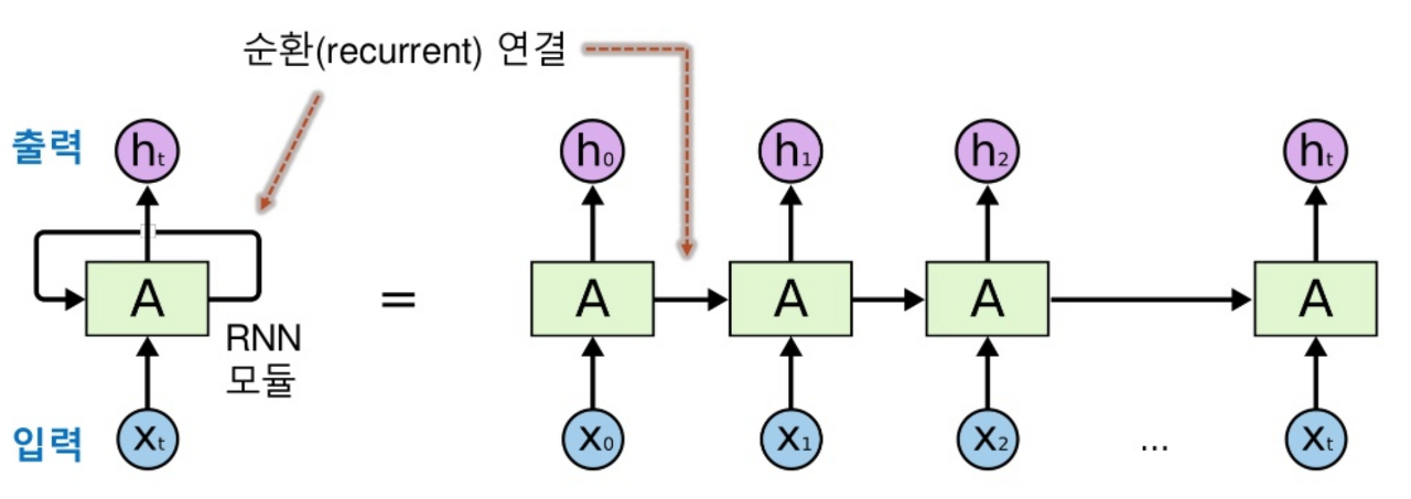
nn.RNN : 기본 인자 값으로 input_size, hidden_size (nn.RNN을 걸치면 나오는 Output), num_layer (층)
output
output[-1] : [sequence, batch_size, hidden_size] 에서 Sequence의 가장 끝
hidden[-1] : [num_layer, batch_size, hidden_size] 에서 num_layer의 가장 끝
https://brunch.co.kr/@linecard/324
GPU 없어서 CPU
device = torch.device('cpu')
class LSTM1(nn.Module):
  def __init__(self, num_classes, input_size, hidden_size, num_layers, seq_length):
    super(LSTM1, self).__init__()
    self.num_classes = num_classes #number of classes
    self.num_layers = num_layers #number of layers
    self.input_size = input_size #input size
    self.hidden_size = hidden_size #hidden state
    self.seq_length = seq_length #sequence length

    self.lstm = nn.LSTM(input_size=input_size, hidden_size=hidden_size,
                      num_layers=num_layers, batch_first=True) #lstm
    self.fc_1 =  nn.Linear(hidden_size, 128) #fully connected 1
    self.fc = nn.Linear(128, num_classes) #fully connected last layer

    self.relu = nn.ReLU()

  def forward(self,x):
    h_0 = Variable(torch.zeros(self.num_layers, x.size(0), self.hidden_size)).to(device) #hidden state
    c_0 = Variable(torch.zeros(self.num_layers, x.size(0), self.hidden_size)).to(device) #internal state
    # Propagate input through LSTM

    output, (hn, cn) = self.lstm(x, (h_0, c_0)) #lstm with input, hidden, and internal state

    hn = hn.view(-1, self.hidden_size) #reshaping the data for Dense layer next
    out = self.relu(hn)
    out = self.fc_1(out) #first Dense
    out = self.relu(out) #relu
    out = self.fc(out) #Final Output

    return out
네트워크 파라미터 구성
num_epochs = 30000 #1000 epochs
learning_rate = 0.00001 #0.001 lr

input_size = 5 #number of features
hidden_size = 2 #number of features in hidden state
num_layers = 1 #number of stacked lstm layers

num_classes = 1 #number of output classes
for epoch in range(num_epochs):
outputs = lstm1.forward(X_train_tensors_final.to(device)) # forward pass
optimizer.zero_grad() # caluclate the gradient, manually setting to 0
# obtain the loss function
loss = loss_function(outputs, y_train_tensors.to(device))
loss.backward() #calculates the loss of the loss function
optimizer.step() #improve from loss, i.e backprop
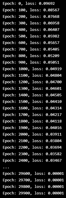
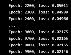
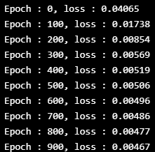
if epoch % 100 == 0:
print("Epoch: %d, loss: %1.5f" % (epoch, loss.item()))