
😎 공부하는 징징알파카는 처음이지?
[Keras] Timeseries anomaly detection using an Autoencoder 본문
👩💻 인공지능 (ML & DL)/ML & DL
[Keras] Timeseries anomaly detection using an Autoencoder
징징알파카 2022. 11. 23. 16:37728x90
반응형
<본 블로그는 keras 의 Timeseries 블로그를 참고해서 공부하며 작성하였습니다 :-)>
https://keras.io/examples/timeseries/timeseries_anomaly_detection/#introduction
Keras documentation: Timeseries anomaly detection using an Autoencoder
Timeseries anomaly detection using an Autoencoder Author: pavithrasv Date created: 2020/05/31 Last modified: 2020/05/31 Description: Detect anomalies in a timeseries using an Autoencoder. View in Colab • GitHub source Introduction This script demonstrate
keras.io
⚡ 1. Setup
import numpy as np
import pandas as pd
from tensorflow import keras
from keras import layers
from matplotlib import pyplot as plt
⚡ 2. Load the data
df_daily_jumpsup_url = "./data/test.csv"
df_daily_jumpsup = pd.read_csv(
    df_daily_jumpsup_url, parse_dates=True
)

print(df_daily_jumpsup.head())
df_daily_jumpsup = df_daily_jumpsup.set_index("insert_date_time")
df_daily_jumpsup.shape
⚡ 3. Visualize the data
- Timeseries data with anomalies
fig, ax = plt.subplots()
df_daily_jumpsup.plot(legend=False, ax=ax)
plt.show()
⚡ 4. Prepare training data
training_mean = df_daily_jumpsup.mean(numeric_only=True)
training_std = df_daily_jumpsup.std(numeric_only=True)
df_training_value = (df_daily_jumpsup - training_mean) / training_std
print("Number of training samples:", len(df_training_value))
- Create sequences
TIME_STEPS = 288

# Generated training sequences for use in the model.
def create_sequences(values, time_steps=TIME_STEPS):
    output = []
    for i in range(len(values) - time_steps + 1):
        output.append(values[i : (i + time_steps)])
    return np.stack(output)


x_train = create_sequences(df_training_value.values)
print("Training input shape: ", x_train.shape)

⚡ 5. Build a model
- input of shape (batch_size, sequence_length, num_features)
model = keras.Sequential(
    [
        layers.Input(shape=(x_train.shape[1], x_train.shape[2])),
        layers.Conv1D(
            filters=32, kernel_size=7, padding="same", strides=2, activation="relu"
        ),
        layers.Dropout(rate=0.2),
        layers.Conv1D(
            filters=16, kernel_size=7, padding="same", strides=2, activation="relu"
        ),
        layers.Conv1DTranspose(
            filters=16, kernel_size=7, padding="same", strides=2, activation="relu"
        ),
        layers.Dropout(rate=0.2),
        layers.Conv1DTranspose(
            filters=32, kernel_size=7, padding="same", strides=2, activation="relu"
        ),
        layers.Conv1DTranspose(filters=1, kernel_size=7, padding="same"),
    ]
)
model.compile(optimizer=keras.optimizers.Adam(learning_rate=0.001), loss="mse")
model.summary()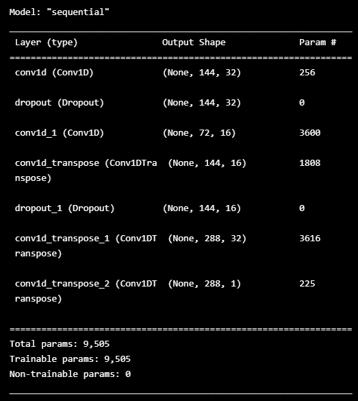
⚡ 6. Train the model
history = model.fit(
    x_train,
    x_train,
    epochs=50,
    batch_size=128,
    validation_split=0.1,
    callbacks=[
        keras.callbacks.EarlyStopping(monitor="val_loss", patience=5, mode="min")
    ],
)
plt.plot(history.history["loss"], label="Training Loss")
plt.plot(history.history["val_loss"], label="Validation Loss")
plt.legend()
plt.show()
⚡ 7. Detecting anomalies
- 훈련 샘플에서 MAE 손실을 찾기
- 최대 MAE 손실 값을 찾음
- 모델이 샘플을 재구성하려고 시도한 것 중 최악
- 이것을 이상 탐지를 위한 임계값으로 만들 것임
- 샘플의 재구성 손실이 이 임계값보다 크면 모델이 익숙하지 않은 패턴을 보고 있다고 추론 할 수 있음
- 이 샘플을 이상 항목으로 표시
# Get train MAE loss.
x_train_pred = model.predict(x_train)
train_mae_loss = np.mean(np.abs(x_train_pred - x_train), axis=1)
plt.hist(train_mae_loss, bins=50)
plt.xlabel("Train MAE loss")
plt.ylabel("No of samples")
plt.show()
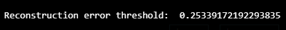
# Get reconstruction loss threshold.
threshold = np.max(train_mae_loss)
print("Reconstruction error threshold: ", threshold)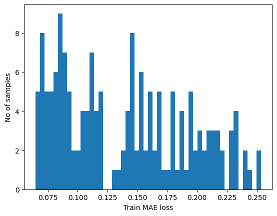
- Compare recontruction
# Checking how the first sequence is learnt
plt.plot(x_train[0])
plt.plot(x_train_pred[0])
plt.show()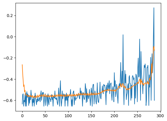
⚡ 8. Prepare test data
df_test_value = (df_daily_jumpsup - training_mean) / training_std
fig, ax = plt.subplots()
df_test_value.plot(legend=False, ax=ax)
plt.show()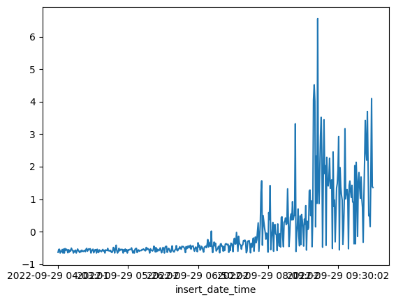
# Create sequences from test values.
x_test = create_sequences(df_test_value.values)
print("Test input shape: ", x_test.shape)
# Get test MAE loss.
x_test_pred = model.predict(x_test)
test_mae_loss = np.mean(np.abs(x_test_pred - x_test), axis=1)
test_mae_loss = test_mae_loss.reshape((-1))
test_mae_loss
plt.hist(test_mae_loss, bins=50)
plt.xlabel("test MAE loss")
plt.ylabel("No of samples")
plt.show()

# Detect all the samples which are anomalies.
anomalies = test_mae_loss > threshold
print("Number of anomaly samples: ", np.sum(anomalies))
print("Indices of anomaly samples: ", np.where(anomalies))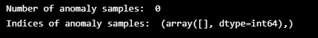
⚡ 9. Plot anomalies
- 난.. 비정상만 있어서 정상친구랑 비정상친구랑 비교하기가 어렵단으 ㅠㅠ
# data i is an anomaly if samples [(i - timesteps + 1) to (i)] are anomalies
anomalous_data_indices = []
for data_idx in range(TIME_STEPS - 1, len(df_test_value) - TIME_STEPS + 1):
    if np.all(anomalies[data_idx - TIME_STEPS + 1 : data_idx]):
        anomalous_data_indices.append(data_idx)
df_subset = df_daily_jumpsup.iloc[anomalous_data_indices]
fig, ax = plt.subplots()
df_daily_jumpsup.plot(legend=False, ax=ax)
df_subset.plot(legend=False, ax=ax, color="r")
plt.show()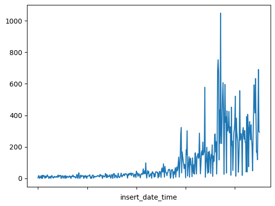
728x90
반응형
'👩💻 인공지능 (ML & DL) > ML & DL' 카테고리의 다른 글
| train validation test set 과의 차이점 (0) | 2022.12.16 |
|---|---|
| 모델 파라미터 batch, epoch, learning rate란? (0) | 2022.12.15 |
| Self-supervised Learning(자기주도학습) 와 Supervised Contrastive Learing (0) | 2022.11.23 |
| 4. 암호화 기법으로 안전한 메시지 전송하기 – “해독 불가능한 암호문을 작성해보자” (0) | 2022.10.20 |
| 3. NLTK로 텍스트 요약하기 – “핵심 문장을 뽑아내고 단어 구름을 만들어보자” (0) | 2022.10.17 |
'👩💻 인공지능 (ML & DL)/ML & DL' Related Articles
more


Comments