
😎 공부하는 징징알파카는 처음이지?
csv 데이터로 미래 예측 LSTM 모델 만들기 본문
728x90
반응형
🦞 전처리 하기 전에 데이터 구경~
🐸1. 여러 폴더 안에 CSV 파일 합치기
import numpy as np # linear algebra
import pandas as pd # data processing, CSV file I/O (e.g. pd.read_csv)
import matplotlib.pyplot as plt
import math as math
%matplotlib inline

import pickle
import os
# Load the data
forder_list = os.listdir("./DATA")
forder_list
csv1 = []
csv2 = []
csv3 = []
csv4 = []
csv5 = []
csv6 = []

for forder in forder_list :
    paths = "./DATA/" + forder + "/"
    # print(paths)
    file_path = sorted(os.listdir(paths))
    # print(file_path)

    csv1.append(paths + file_path[0])
    csv2.append(paths + file_path[1])
    csv3.append(paths + file_path[2])
    csv4.append(paths + file_path[3])
    csv5.append(paths + file_path[4])
    csv6.append(paths + file_path[5])
🐸2. 같은 csv 끼리 하나의 dataframe으로 concat 하기 (axis = 0)
allData = [] # 읽어 들인 csv파일 내용을 저장할 빈 리스트를 하나 만든다

for file in csv1:
    df = pd.read_csv(file) # for구문으로 csv파일들을 읽어 들인다
    allData.append(df) # 빈 리스트에 읽어 들인 내용을 추가한다
dataCombine = pd.concat(allData, axis=0, ignore_index=True)
🦞 시각화
fig = plt.figure()   #figure객체를 선언해 도화지(그래프) 객체 생성**
ax = fig.add_subplot() ## 그림 뼈대(프레임) 생성  #축을 그려줌**
#figure()객체에 하위 그래프 subplot를 추가. add_subplot 매서드를 이용해 축을 그려줘야 함
# 1, 1, 1의 뜻 : nrows(행), nclos(열), index(그래프가 그려지는 좌표)


for i in range(2, 15) :
    # 특정열 Plot 변환
    plt.title(dataCombine.columns[i])
    plt.plot(dataCombine["insert_date_time"], dataCombine.iloc[:, i], color='r')

    # 생성된 Plot 출력
    plt.show()
데이터가 너무 많은 것 같아서,
시간 별로 SUM 해서 다시 데이터 합쳐보기
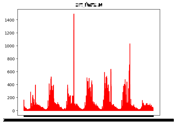
🦞 데이터 전처리
🐸 1. 같은 insert_data_time 별로 묶어서 sum 하기 -> 데이터 줄임
dataCombine2 = dataCombine.groupby(["insert_date_time"], as_index=True).sum()
dataCombine2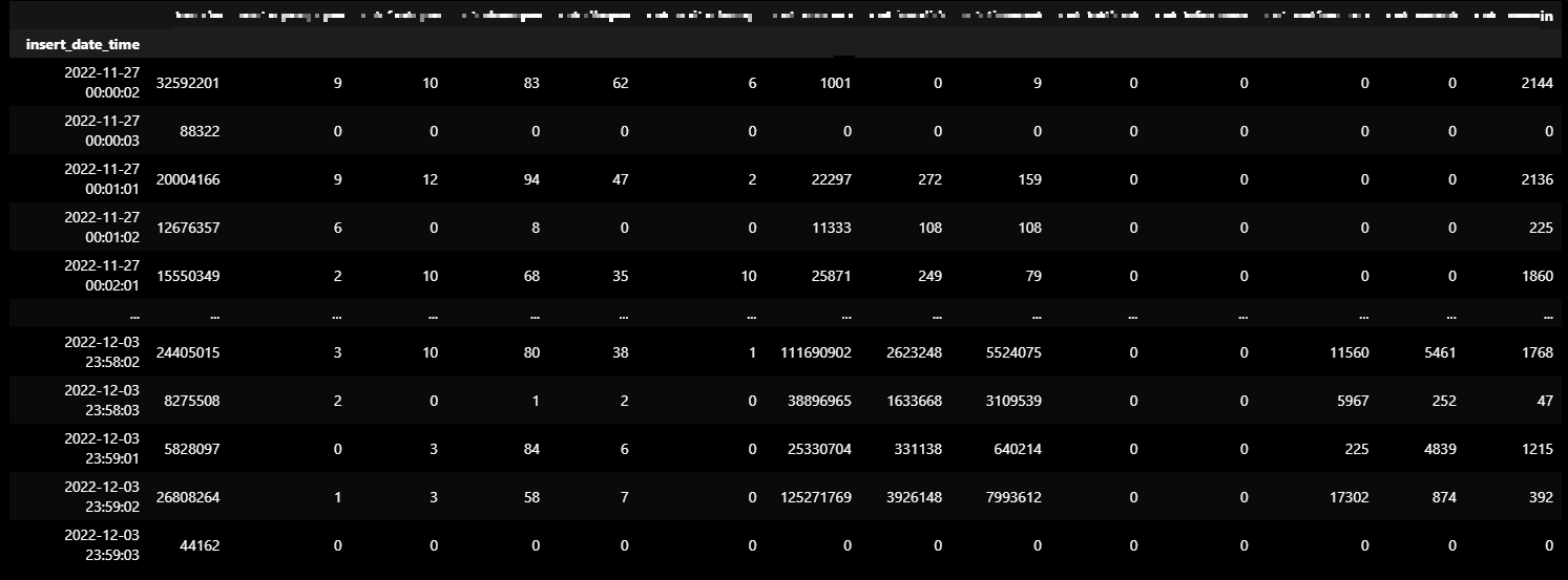
🐸 2. 데이터 스케일링 하기 위해 준비하기
dataCombine2_temp = dataCombine2.reset_index(drop=True)🦞 시각화
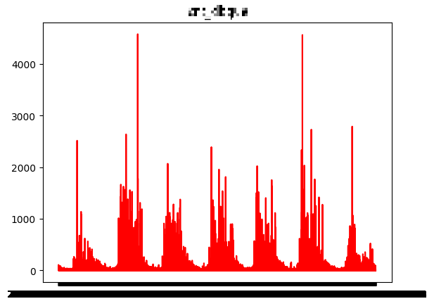
fig = plt.figure()   #figure객체를 선언해 도화지(그래프) 객체 생성**
ax = fig.add_subplot() ## 그림 뼈대(프레임) 생성  #축을 그려줌**
#figure()객체에 하위 그래프 subplot를 추가. add_subplot 매서드를 이용해 축을 그려줘야 함
# 1, 1, 1의 뜻 : nrows(행), nclos(열), index(그래프가 그려지는 좌표)


for i in range(1, 14) :
    # 특정열 Plot 변환
    plt.title(dataCombine2_temp.columns[i])
    plt.plot(dataCombine2.index, dataCombine2_temp.iloc[:, i], color='r')

    # 생성된 Plot 출력
    plt.show()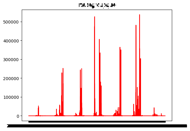

🦞 모델 만들기
🐸 1. 0 데이터 지우고, 주기성 가지는 그래프들만 모아서 LSTM 모델 훈련하기
dataCombine3_temp = dataCombine2_temp.drop(["필요없는거", '0 데이터 뿐', '0 데이터 뿐', '불규칙'], axis = 1)
dataCombine3_temp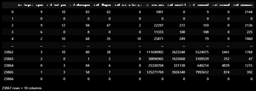
🐸 2. 정규화
!pip install -U sklearn
from sklearn.preprocessing import MinMaxScaler

scaler = MinMaxScaler()

scale_cols = dataCombine3_temp.columns
dataCombine3_temp_scaled = scaler.fit_transform(dataCombine3_temp)
dataCombine3_temp_scaled = pd.DataFrame(dataCombine3_temp_scaled)
dataCombine3_temp_scaled.columns = scale_cols

dataCombine3_temp_scaled
🐸 3. 시계열 데이터의 데이터셋 분리
- 시계열 데이터의 데이터셋은 보통 window_size
- window_size는 과거 기간의 주가 데이터에 기반하여 다음날의 종가를 예측할 것인가를 정하는 parameter
- 만약 과거 20일을 기반으로 내일 데이터를 예측한다라고 가정하면 window_size=20이 되는 것
TEST_SIZE = 200
WINDOW_SIZE = 20

train = dataCombine3_temp_scaled[:-TEST_SIZE]
test = dataCombine3_temp_scaled[-TEST_SIZE:]
def make_dataset(data, label, window_size=20):
feature_list = []
label_list = []
for i in range(len(data) - window_size):
feature_list.append(np.array(data.iloc[i:i+window_size]))
label_list.append(np.array(label.iloc[i+window_size]))
return np.array(feature_list), np.array(label_list)
🐸 4. 훈련, 테스트 데이터 나누기
from sklearn.model_selection import train_test_split

feature_cols = ['routegroupque', 'cnt_fastque', 'cnt_slowque', 'cnt_dbque',
       'cnt_waitackmap', 'cnt_success', 'cnt_invalid', 'cnt_timeout',
       'cnt_resent', 'cnt_onemin']
label_cols = ['cnt_timeout']

train_feature = train[feature_cols]
train_label = train[label_cols]

train_feature, train_label = make_dataset(train_feature, train_label, 20)

x_train, x_valid, y_train, y_valid = train_test_split(train_feature, train_label, test_size=0.2)
x_train.shape, x_valid.shape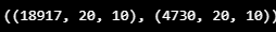
test_feature = test[feature_cols]
test_label = test[label_cols]

test_feature.shape, test_label.shape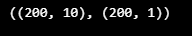
test_feature, test_label = make_dataset(test_feature, test_label, 20)
test_feature.shape, test_label.shape
🐸 5. LSTM 모델
from keras.models import Sequential
from keras.layers import Dense
from keras.callbacks import EarlyStopping, ModelCheckpoint
from keras.layers import LSTM

model = Sequential()
model.add(LSTM(16,
               input_shape=(train_feature.shape[1], train_feature.shape[2]),
               activation='relu',
               return_sequences=False)
          )

model.add(Dense(1))
import os
model.compile(loss='mean_squared_error', optimizer='adam')
early_stop = EarlyStopping(monitor='val_loss', patience=5)
model_path = 'model'
filename = os.path.join(model_path, 'tmp_checkpoint.h5')
checkpoint = ModelCheckpoint(filename, monitor='val_loss', verbose=1, save_best_only=True, mode='auto')
history = model.fit(x_train, y_train,
epochs=200,
batch_size=16,
validation_data=(x_valid, y_valid),
callbacks=[early_stop, checkpoint])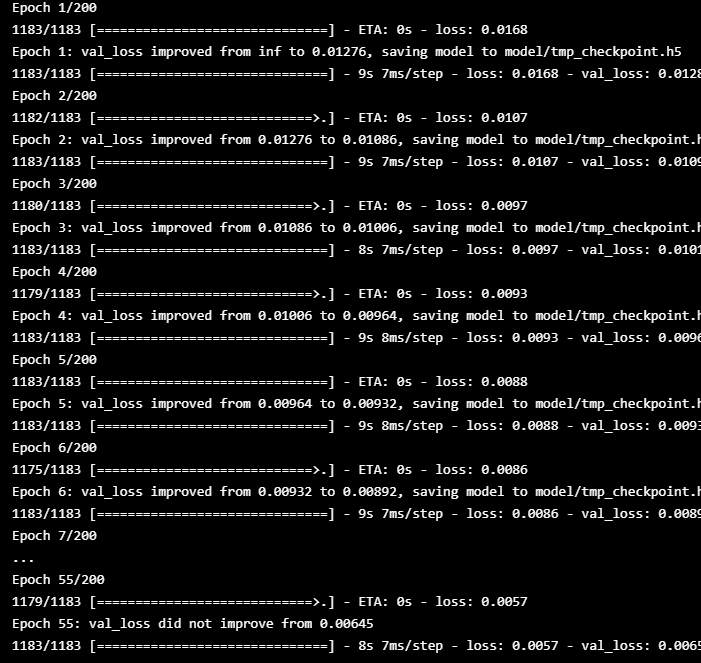
model.load_weights(filename)
pred = model.predict(test_feature)

pred.shape
plt.figure(figsize=(12, 9))
plt.plot(test_label, label = 'actual')
plt.plot(pred, label = 'prediction')
plt.legend()
plt.show()
728x90
반응형
'👩💻 인공지능 (ML & DL) > Serial Data' 카테고리의 다른 글
| Dash와 Python을 사용하여 사용자 입력 기반 그래프 (0) | 2022.11.14 |
|---|---|
| Dash와 Python을 사용하여 실시간 업데이트 그래프를 생성 (0) | 2022.11.14 |
| CNN-LSTM 으로 시계열 분석하기 (0) | 2022.11.04 |
| Serial Data 장애 예측/감지 LSTM & Conv 모델 (0) | 2022.10.28 |
| 코로나 확진 예방을 위해 시계열(Time-Series) 데이터로 LSTM 예측 모델만들기 (1) | 2022.10.26 |
'👩💻 인공지능 (ML & DL)/Serial Data' Related Articles
more


Comments