
😎 공부하는 징징알파카는 처음이지?
[음성] 음성인식 음악분류 & 추천 알고리즘 본문
220131 작성
<본 블로그는 조녁 코딩일기를 참고해서 공부하며 작성하였습니다>
https://jonhyuk0922.tistory.com/114
[Librosa] 음성인식 기초 및 음악분류 & 추천 알고리즘
안녕하세요~ 27년차 진로탐색꾼 조녁입니다!! 오늘은 음성파일을 인식하고 거기서 특징추출하는 기초적인 내용부터 추출한 특징들을 통해 노래의 장르를 분류하는 모델과 비슷한 장르의 노래를
jonhyuk0922.tistory.com
https://newsight.tistory.com/294
음성인식 기초 이해하기
# 발음기호와 문자표현 - phoneme: 음소, 가장 작은 소리의 단위. 쉽게 말해 영어사전의 발음기호를 생각하면 된다. - grapheme: 자소(=문자소), 가장 작은 문자의 단위. 발음기호로 표현되기 이전의 원
newsight.tistory.com
1. 소리
: 공기에 주기적인 진동(앞뒤로의 수축/팽창)이 발생해야만 소리
: 공기를 매질로하는 파동 에너지가 바로 소리의 정체
: 파동의 진동수가 작으면 낮은 에너지를 가진 저음
: 진동수가 크면 많은 에너지를 가진 고음
2. Wav 파일
: 소리 파동의 높이 값(float형)을 일정한 시간 간격(sampling rate)마다 기록한 실수의 배열
: 저장 방식을 PCM(Pulse-Code Modulation)
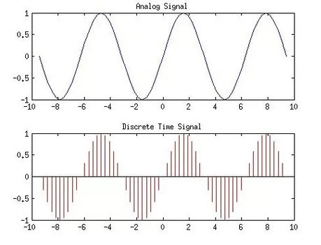
: 숫자로 이루어짐
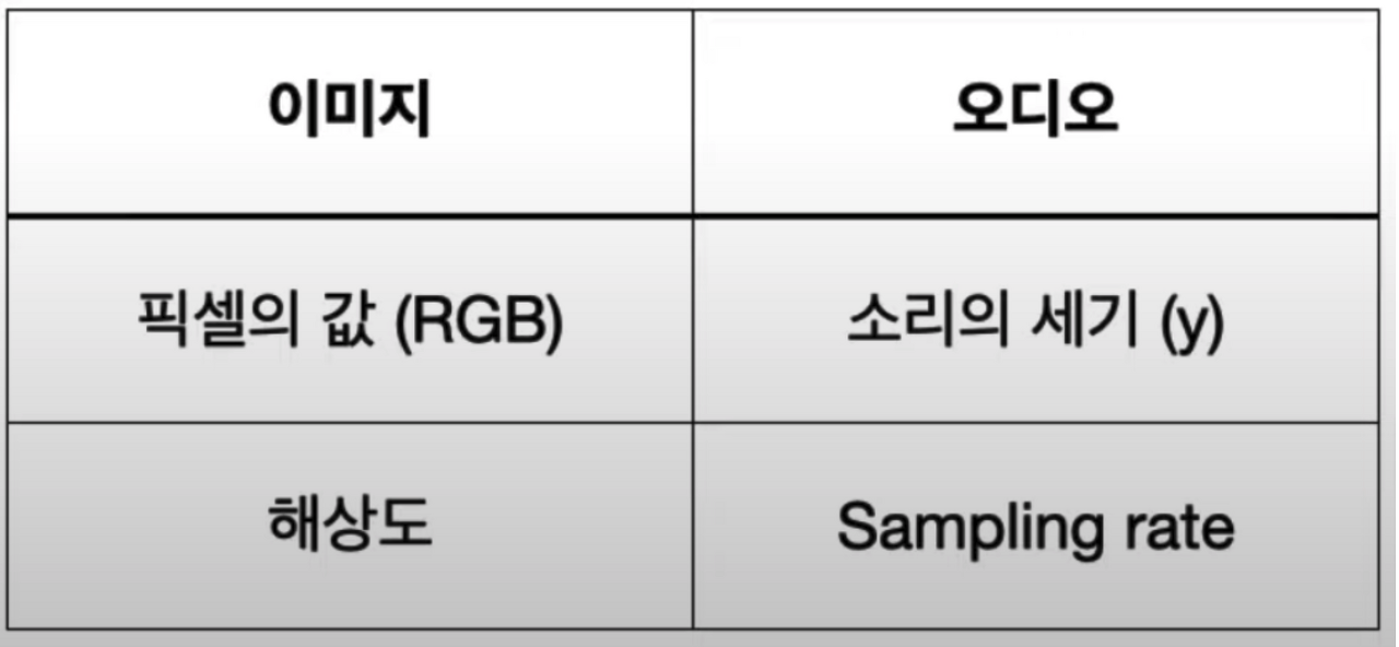
- y : 소리가 떨리는 세기(진폭)를 시간 순서대로 나열한 것
- Sampling rate: 1초당 샘플의 개수, 단위 1초당 Hz 또는 kHz
- Mono vs Stereo
: Left-Right 마이크 2개에서 들어온 소리(2개의 mono)를 녹음해서 한 번에 저장한 것을 스테레오
- Sampling rate
: data point의 x축 해상도
: 1초에 몇번이나 data point를 찍을지이다.
- Bit depth
: data point의 y축 해상도
: 각 점들의 높이(amplitude)를 구분할 수 있는 해상도
- Bit rate
: Sampling rate * Bit depth
: 초당 bits전송량
3. 소리 파일 분석 ( with kaggle )
- 1) 데이터셋 로드
import librosa

# librosa.load() : 오디오 파일을 로드
y , sr = librosa.load('Data/genres_original/reggae/reggae.00036.wav')

print(y)
print(len(y))
print(y.shape)
print('Sampling rate (Hz): %d' %sr)
print('Audio length (seconds): %.2f' % (len(y) / sr))
#음악의 길이(초) = 음파의 길이/Sampling rate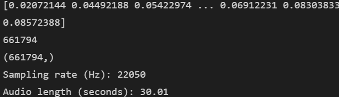
- 2) 음악 들어보기
import IPython.display as ipd
ipd.Audio(y, rate=sr)
- VS code 에서는 안들린당..
- colab 으로 돌리니까 나옸ㅏ땨!
- 3) 음악 그래프
- 2D 그래프
import matplotlib.pyplot as plt
import librosa.display

plt.figure(figsize =(16,6))
librosa.display.waveplot(y=y,sr=sr)
plt.show()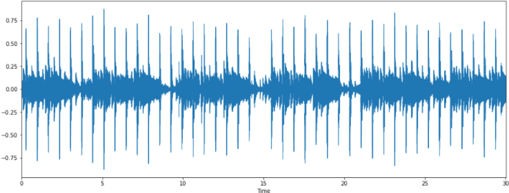
- Fourier Transform(푸리에 변환)
: 시간 영역 데이터를 주파수 영역으로 변경
: time(시간) domain -> frequency(진동수)
- y축 : 주파수(로그 스케일)
- color축 : 데시벨(진폭)
import numpy as np

# n_fft : window size
# 음성의 길이를 얼마만큼으로 자를 것인가? => window
Fourier = np.abs(librosa.stft(y, n_fft=2048, hop_length=512))

print(Fourier.shape)

plt.figure(figsize=(16,6))
plt.plot(Fourier)
plt.show()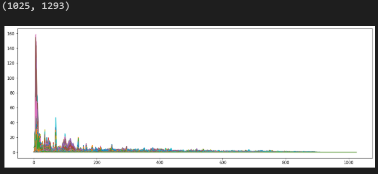
- Spectogram
: 시간에 따른 신호 주파수의 스펙트럼 그래프
# amplitude(진폭) -> DB(데시벨)로 바꿔라
DB = librosa.amplitude_to_db(Fourier, ref=np.max)

plt.figure(figsize=(16,6))
librosa.display.specshow(DB,sr=sr, hop_length=512, x_axis='time', y_axis='log')
plt.colorbar()
plt.show()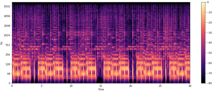
- Mel Spectogram
: Spectogram의 y축을 Mel Scale로 변환한 것
Mel = librosa.feature.melspectrogram(y, sr=sr)
Mel_DB = librosa.amplitude_to_db(Mel, ref=np.max)

plt.figure(figsize=(16,6))
librosa.display.specshow(Mel_DB, sr=sr,hop_length=512, x_axis='time',y_axis='log')
plt.colorbar()
plt.show()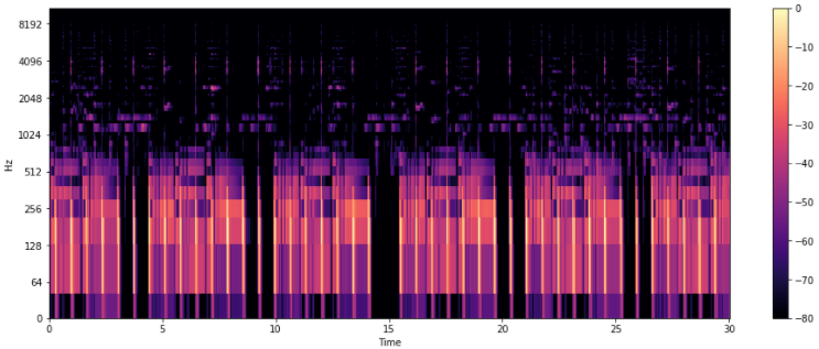
- 4) 레게 VS 클래식 비교
y, sr = librosa.load('Data/genres_original/classical/classical.00036.wav')
y, _ = librosa.effects.trim(y)

S = librosa.feature.melspectrogram(y, sr=sr)
S_DB = librosa.amplitude_to_db(S, ref=np.max)

plt.figure(figsize=(16,6))
librosa.display.specshow(S_DB, sr=sr,hop_length=512, x_axis='time',y_axis='log')
plt.colorbar()
plt.show()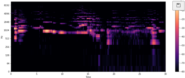
- 5) 오디오 특성 추출(Audio Feature Extraction)
- Tempo(BPM)
tempo , _ = librosa.beat.beat_track(y,sr=sr)
print(tempo)
- Zero Crossing Rate
: 음파가 양에서 음으로 또는 음에서 양으로 바뀌는 비율
# 0이 되는 선을 지나친 횟수
zero_crossings = librosa.zero_crossings(y, pad=False)

print(zero_crossings)
print(sum(zero_crossings)) # 음 <-> 양 이동한 횟수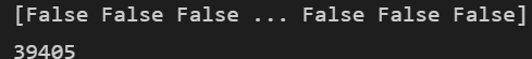
: Zero Crossing은 0이 되는 선을 지나친 횟수
n0 = 9000
n1 = 9080

plt.figure(figsize=(16,6))
plt.plot(y[n0:n1])
plt.grid()
plt.show()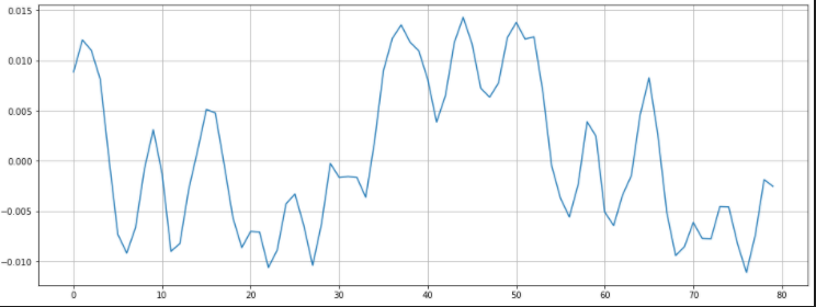
: 그래프 0 이하로 찍는거 보면 약 11 개?
 #n0 ~ n1 사이 zero crossings
zero_crossings = librosa.zero_crossings(y[n0:n1], pad=False)
print(sum(zero_crossings))
- 6) 특징 추출
- 1) Harmonic and Percussive Components
- Percussives: 리듬과 감정을 나타내는 충격파
- Harmonics : 사람의 귀로 구분할 수 없는 특징들(음악의 색깔)
y_harm, y_perc = librosa.effects.hpss(y)

plt.figure(figsize=(16,6))
plt.plot(y_harm, color='b')
plt.plot(y_perc, color='r')
plt.show()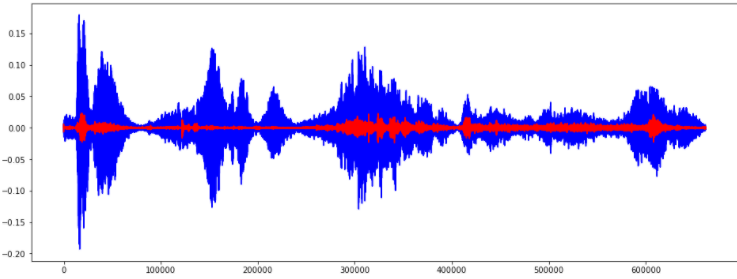
- 2) Spectral Centroid
: 소리를 주파수 표현했을 때, 주파수의 가중평균을 계산하여 소리의 "무게 중심"이 어딘지를 알려주는 지표
spectral_centroids = librosa.feature.spectral_centroid(y, sr=sr)[0]

#Computing the time variable for visualization
frames = range(len(spectral_centroids))

# Converts frame counts to time (seconds)
t = librosa.frames_to_time(frames)

import sklearn
def normalize(x, axis=0):
# sk.minmax_scale() : 최대 최소를 0 ~ 1 로 맞춰준다.
  return sklearn.preprocessing.minmax_scale(x, axis=axis)

plt.figure(figsize=(16,6))
librosa.display.waveplot(y, sr=sr, alpha=0.5, color='b')
plt.plot(t, normalize(spectral_centroids), color='r')
plt.show()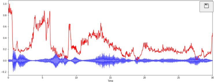
- 3) Spectral Rolloff
: 총 스펙트럴 에너지 중 낮은 주파수(85% 이하)에 얼마나 많이 집중되어 있는가
: 신호 모양을 측정
spectral_rolloff = librosa.feature.spectral_rolloff(y, sr=sr)[0]

plt.figure(figsize=(16,6))
librosa.display.waveplot(y,sr=sr,alpha=0.5,color='b')
plt.plot(t, normalize(spectral_rolloff),color='r')
plt.show()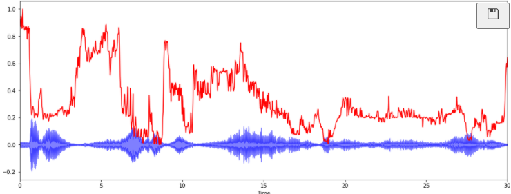
- 4) Mel-Frequency Cepstral Coefficients(MFCCs)
: MFCCs는 특징들의 작은 집합(약 10-20)으로 스펙트럴 포곡선의 전체적인 모양을 축약
: 사람의 청각 구조를 반영하여 음성 정보 추출
1. 전체 오디오 신호를 일정 간격으로 나누고 푸리에 변환을 거쳐 스펙트로그램을 구합니다.
2. 각 스펙트럼의 제곱인 파워 스펙트로그램에 Mel scale filter bank를 사용해 차원 수를 줄입니다.
3. cepstral 분석을 적용해 MFCC를 구합니다.
출처: https://tech.kakaoenterprise.com//66
mfccs = librosa.feature.mfcc(y, sr=sr)
mfccs = normalize(mfccs,axis=1)

print('mean : %.2f' % mfccs.mean())
print('var : %.2f' % mfccs.var())

plt.figure(figsize=(16,6))
librosa.display.specshow(mfccs,sr=sr, x_axis='time')
plt.show()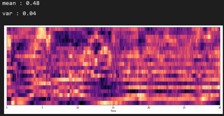
- Chroma Frequencies
: 크로마는 인간 청각이 옥타브 차이가 나는 주파수를 가진 두 음을 유사음으로 인지
: 크로마 특징은 음악의 흥미롭고 강렬한 표현
chromagram = librosa.feature.chroma_stft(y, sr=sr, hop_length=512)

plt.figure(figsize=(16,6))
librosa.display.specshow(chromagram,x_axis='time', y_axis='chroma', hop_length=512)
plt.show()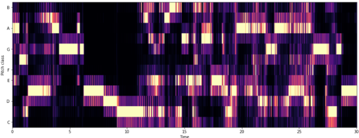
4. 음악 장르 분류 ( with kaggle )
- 1) 데이터셋 로드
from sklearn.model_selection import train_test_split
import numpy as np
import pandas as pd

from sklearn.metrics import classification_report
from sklearn.tree import DecisionTreeClassifier
from sklearn.ensemble import RandomForestClassifier
from sklearn import svm
from sklearn.svm import SVC
from sklearn.linear_model import SGDClassifier
from sklearn.linear_model import LogisticRegression

from sklearn.pipeline import Pipeline, make_pipeline
from sklearn.preprocessing import StandardScaler
from sklearn.preprocessing import MinMaxScaler

from sklearn.metrics import confusion_matrix, classification_report
from sklearn.metrics import accuracy_score, precision_score, recall_score, f1_score, roc_auc_score
from sklearn.metrics import roc_curve, auc

from sklearn.model_selection import cross_val_score
from sklearn.model_selection import cross_val_predict
from sklearn.model_selection import GridSearchCV

import matplotlib.pyplot as plt
%matplotlib inline
import seaborn as sns
sns.set_style('whitegrid')  # 그래프 테두리 모두 제거
df = pd.read_csv('Data/features_3_sec.csv')
df.head()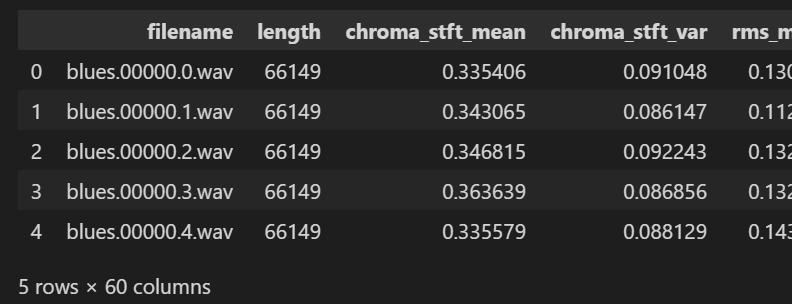
- 2) 데이터 전처리
X = df.drop(columns=['filename','length','label']) # 필요 없는것!
y = df['label'] #장르명

scaler = MinMaxScaler()   # scale 0~1 조정
np_scaled = scaler.fit_transform(X)

X = pd.DataFrame(np_scaled, columns=X.columns)

X.head()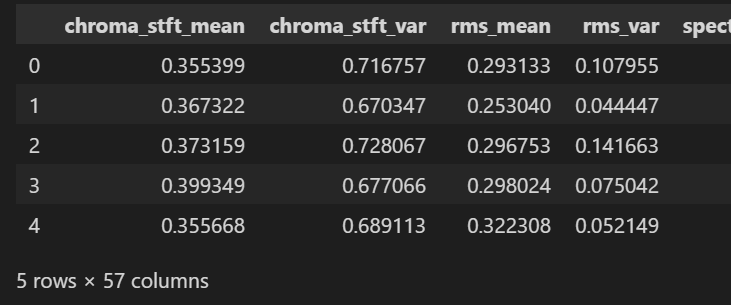
- 3) Train, Test 분할
X_train , X_test , y_train, y_test = train_test_split(X,y , test_size=0.2, random_state=42)

print(X_train.shape, y_train.shape)
print(X_test.shape, y_test.shape)
- 4) 모델 구축
- xgboost
d
from xgboost import XGBClassifier
from sklearn.metrics import accuracy_score

xgb = XGBClassifier(n_estimators=100, learning_rate=0.05) #1000개의 가지, 0.05 학습률

xgb.fit(X_train, y_train) #학습

print("xgb Test Accuarcy : {}%".format(round(xgb.score(X_test, y_test) * 100, 2)))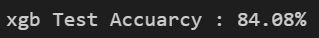
- Logistic Regression
lr = LogisticRegression(solver = "lbfgs")
lr.fit(X_train, y_train)

print("lr Test Accuarcy : {}%".format(round(lr.score(X_test, y_test) * 100, 2)))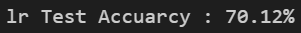
- RandomForest
rf = RandomForestClassifier(n_estimators = 100, random_state = 42)
rf.fit(X_train, y_train)

print("rf Test Accuarcy : {}%".format(round(rf.score(X_test, y_test) * 100, 2)))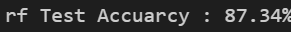
- Decision Tree
tree = DecisionTreeClassifier()
params = {
    'max_depth' : [6, 8, 10, 12, 16, 20, 24],
    'min_samples_split' : [16, 24]
}

grid_dt = GridSearchCV(tree, param_grid=params, scoring='accuracy', cv=5, verbose=1)
grid_dt.fit(X_train, y_train)

print('최상의 교차검증 정확도 {:.2f}'.format(grid_dt.best_score_))
print("rf Test Accuarcy : {}%".format(round(grid_dt.score(X_test, y_test) * 100, 2)))
print('최적의 매개변수 : {}'.format(grid_dt.best_params_))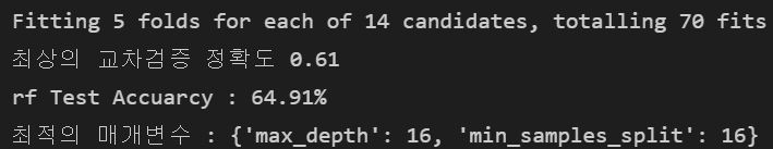
- 5) Confusion Matrix
y_preds = rf.predict(X_test) #검증

cm = confusion_matrix(y_test,y_preds)

plt.figure(figsize=(16,9))
sns.heatmap(
    cm,
    annot=True,
    xticklabels=["blues","classical","country","disco","hiphop","jazz","metal","pop","reggae","rock"],
    yticklabels=["blues","classical","country","disco","hiphop","jazz","metal","pop","reggae","rock"]
)
plt.show()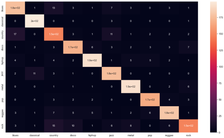
- 6) Confusion Matrix
for feature, importance in zip(X_test.columns, rf.feature_importances_):
  print('%s: %.2f' % (feature, importance))   #어떤 특징이 중요했는지 보여줌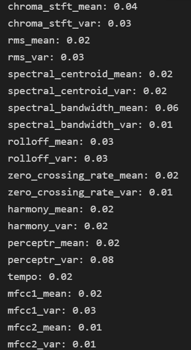
5. 노래 추천
- 1) 데이터 로드
df_30 = pd.read_csv('Data/features_30_sec.csv', index_col='filename')

labels = df_30[['label']]
df_30 = df_30.drop(columns=['length','label'])

df_30_scaled = StandardScaler().fit_transform(df_30)    #평균 0 , 표준편차 1

df_30 = pd.DataFrame(df_30_scaled, columns=df_30.columns)

df_30.head()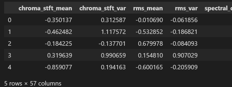
- 2) 유사도 설정
from sklearn.metrics.pairwise import cosine_similarity

# 벡터의 유사도 , 즉 벡터간의 각도를 통해 추정 cos0 =1 이므로 1에 가까울 수록 유사
# cos180 = -1 이므로 -1에 가까울 수록 다르다.
similarity = cosine_similarity(df_30)

sim_df = pd.DataFrame(similarity, index=labels.index, columns=labels.index)

sim_df.head()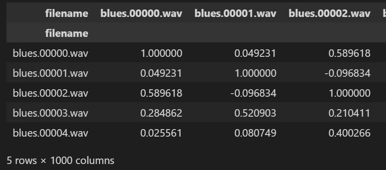
- +) 함수화
def find_similar_songs(name, n=5):
  series = sim_df[name].sort_values(ascending=False)

  series = series.drop(name)

  return series.head(n).to_frame()

find_similar_songs('rock.00000.wav')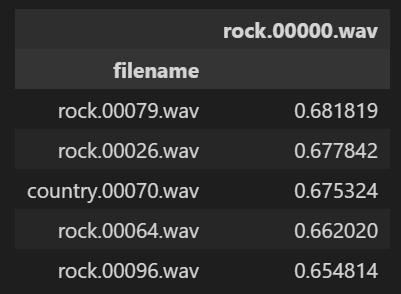
'👩💻 인공지능 (ML & DL) > ML & DL' 카테고리의 다른 글
| [Deep Learning]_3_미분 기초 (2) (0) | 2022.02.01 |
|---|---|
| [Deep Learning]_2_미분 기초 (1) (0) | 2022.02.01 |
| [CNN]_Convolution 과정 (0) | 2022.01.29 |
| [DEEPNOID 원포인트레슨]_10_GAN (0) | 2022.01.28 |
| [DEEPNOID 원포인트레슨]_9_AutoEncoder & GAN (0) | 2022.01.28 |


