
😎 공부하는 징징알파카는 처음이지?
다변량 시계열 데이터 2 (Multivariate Time Series Data) 본문
👩💻 인공지능 (ML & DL)/Serial Data
다변량 시계열 데이터 2 (Multivariate Time Series Data)
징징알파카 2022. 9. 30. 09:54728x90
반응형
220930 작성
<본 블로그는 ysyblog 님의 블로그를 참고해서 공부하며 작성하였습니다>
https://ysyblog.tistory.com/298
[시계열분석] 다변량 선형 확률과정 - VAR & IRP (백터자기회귀과정, 임펄스응답함수)
다변량 선형 확률과정 필요성 단변량 시계열(Simple/Multiple포함)은 종속변수(Y_t)가 독립변수들에만! 영향을 받는다는 큰 가정 존재 현실적으론 종속변수와 독립변수는 상호 영향을 주고받음 예시:
ysyblog.tistory.com
1️⃣ 다변량 시계열
- 종속변수(Y_t)가 독립변수들에만 영향 받음
- 2차원(소득, 지출 : 종속변수) 과거 1시점가지만을 고려하는 벡터자기회귀 알고리즘

💗 벡터자기회귀 모형
1) VAR 알고리즘
- 평균 벡터와 공분산 벡터가 시차에만 의존하고 각각의 절대위치에 독립적인 정상성 시계열
2) 임펄스 응답 함수
- 여러개의 시계열 상호 상관관계를 기반으로 각각의 변수가 다른 변수에 어떤 영향을 주는지 임펄스 반응 함수로 알 수 있음
- 임펄스 : 어떤 시계열이 t = 0 일 때 1이고, t < 0 or t > 0 일 때 0
- 임펄스 형태의 시계열이 다른 시계열에 미치는 영향을 시간에 따라 표시
2️⃣ 코드 구현
💗 데이터 로딩 및 시각화
import pandas as pd
import numpy as np
import matplotlib.pyplot as plt
import statsmodels
import statsmodels.api as sm

raw = sm.datasets.macrodata.load_pandas().data
dates_info = raw[['year', 'quarter']].astype(int).astype(str)
raw.index = pd.DatetimeIndex(sm.tsa.datetools.dates_from_str(dates_info['year'] + 'Q'+ dates_info['quarter']))
raw_use = raw.iloc[:, 2:5]- 실제 GDP = 실제 CON(소비) + 실제 INV(투자)
raw_use.plot(subplots = True, figsize = (12, 5))
plt.tight_layout()
plt.show()
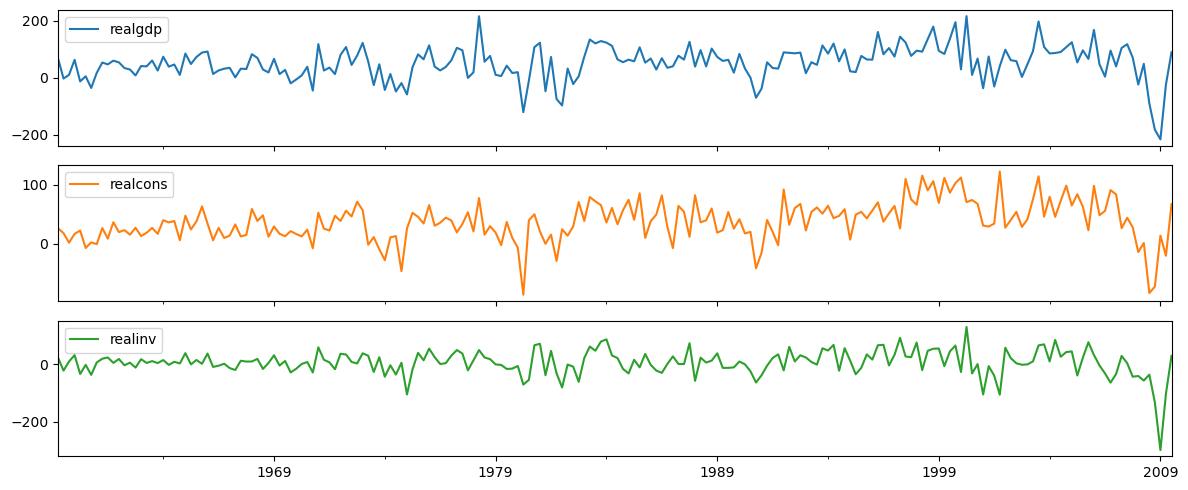
raw_use.diff(1).dropna().plot(subplots = True, figsize = (12, 5))
plt.tight_layout()
plt.show()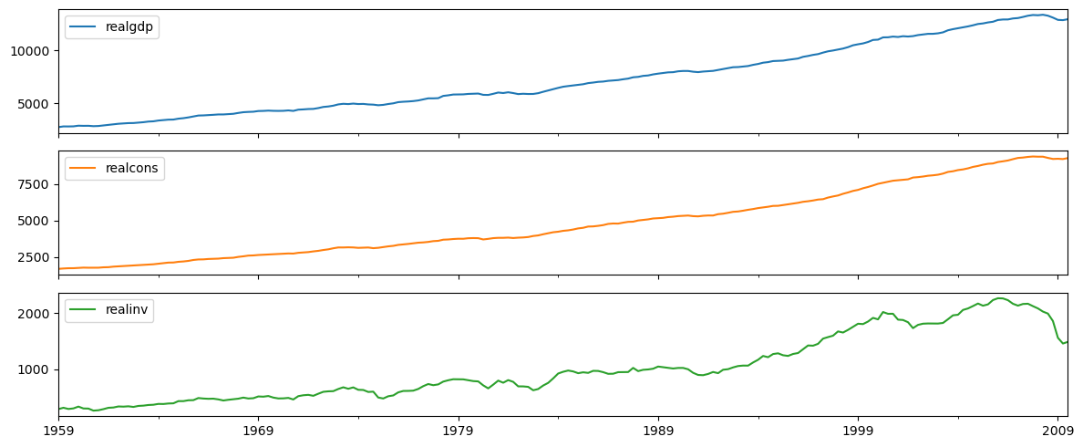
💗 VAR 모형
- realgdp : realgdp, realcon, realinv 의 시차 L1 모두와 realcon의 시차 L2에 영향
- realcon : realgdp, realcon, realinv 에 시차 L1, L2 모두 영향
- realinv : realgdp, realcon, realinv 에 시차 L1 만 영향
- realcon, realgdp, realinv 순으로 가장 다른 변수에 영향 많이 받음
raw_use_return = raw_use.diff(1).dropna()
fit = sm.tsa.VAR(raw_use_return).fit(maxlags = 2)
display(fit.summary())
💗 모형 예측 및 시각화
forecast_num = 20

# 점추정
# pre_var = fit.forecast(fit.model.endog[-1:], steps = forecast_num)

# 구간추정
# pre_var_ci = fit.forecast_interval(fit.model.endog[-1:], steps = forecast_num)

fit.plot_forecast(forecast_num)
plt.tight_layout()
plt.show()
- 임펄스 반응 함수
- realgdp -> realgdp : 단기적으로 음수로 바뀌지만 0으로 수렴
- realgdp -> realcons : gdp가 증가, 소비가 감소하다가 늘어남
- realinv -> realcons : 실제 투자가 증가하면서 실제 소비 증가하다가 0으로 수렴
- realcon -> realgdp : 소비가 증가하면 실제 gdp가 상당히 증가하다가 0으로 수렴
- realinv -> realgdp : 투자가 증가하면 실제 gdp가 소폭 증가하다가 0으로 수렴
fit.irf(forecast_num).plot()
plt.tight_layout()
plt.show()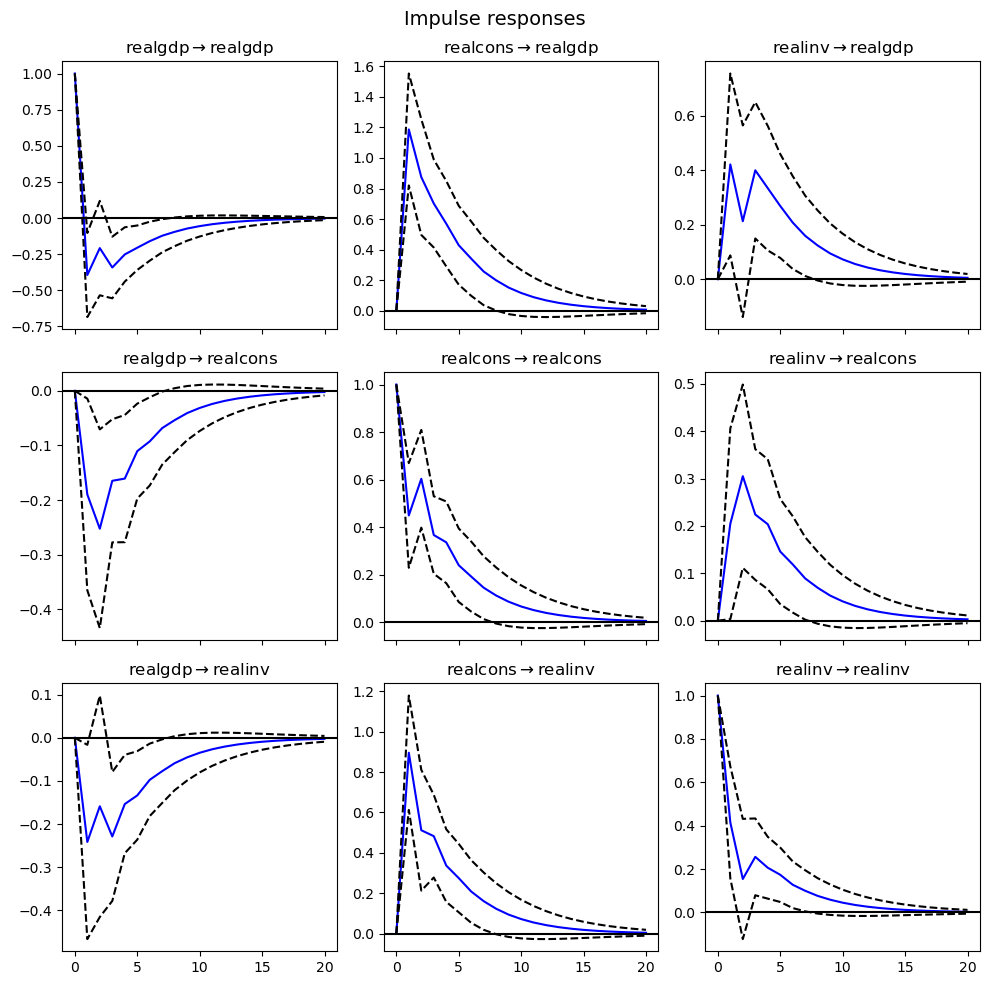
💗 잔차진단
fit.plot_acorr()
plt.tight_layout()
plt.show()

728x90
반응형
'👩💻 인공지능 (ML & DL) > Serial Data' 카테고리의 다른 글
| Time series 시계열 데이터 분류하기 (0) | 2022.10.06 |
|---|---|
| [교과서 리뷰] Forecasting: Principles and Practice (1) | 2022.10.05 |
| 자기 상관(AutoCorrelation)이 강한 시계열 데이터 학습하기 (1) | 2022.09.28 |
| 시계열 데이터 분석 순서 (Time Series Analysis Order) (0) | 2022.09.28 |
| 다변량 시계열 데이터 1 (Multivariate Time Series Data) (0) | 2022.09.28 |
'👩💻 인공지능 (ML & DL)/Serial Data' Related Articles
more


Comments