
😎 공부하는 징징알파카는 처음이지?
[FuncAnimation] 2. 단일변량 그래프를 만들어서 GUI로 시각화하기 본문
👩💻 인공지능 (ML & DL)/Serial Data
[FuncAnimation] 2. 단일변량 그래프를 만들어서 GUI로 시각화하기
징징알파카 2022. 10. 24. 15:06728x90
반응형
221024 작성
<본 블로그는 ahnig 님의 블로그를 참고해서 공부하며 작성하였습니다>
[keras, TF2.0] 온도 데이터, 시계열 예측하기 (Time Series Forecasting)
시계열 예측(Time Series Forecasting) Licensed under the Apache License, Version 2.0 (the "License") MIT License https://www.tensorflow.org/tutorials/structured_data/time_series RNN(Recurrent Neural..
ahnjg.tistory.com
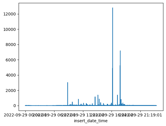
😊 csv 파일을 받아서 실시간 그래프를 만들어보자
- csv 데이터 스케일 조정
- 최근 데이터로 미래온도 예측
- LSTM으로 미래온도 예측
# 1. 단일변량 그래프
## https://operstu1.tistory.com/97
import random
from itertools import count
import pandas as pd
import numpy as np
import matplotlib.pyplot as plt
from matplotlib.animation import FuncAnimation
from pandas.core.indexes import interval
import tensorflow as tf
import matplotlib as mpl
import os
TRAIN_SPLIT = 4000 # 4558 rows
tf.random.set_seed(13)
def load_file() :
# 데이터 로드
data = pd.read_csv("/home/ubuntu/FPDS/20220929/TESTTEST.csv")
# insert_date_time 를 기준으로 집계 합
temp = data.groupby(["insert_date_time"], as_index=False).sum()
# 단일 변수 선택
uni_temp = temp['cnt_item']
uni_temp.index = temp['insert_date_time']
return uni_temp
def scaling(uni_temp) :
# 데이터 값에 평균값을 빼고 표준편차를 나누는 데이터 표준화 (Standardization)
uni_temp = uni_temp.values
uni_train_mean = uni_temp[:TRAIN_SPLIT].mean()
uni_train_std = uni_temp[:TRAIN_SPLIT].std()
uni_data = (uni_temp - uni_train_mean)/(uni_train_std)
return uni_data
def univariate_data(dataset, start_index, end_index, history_size, target_size):
data=[]
labels=[]
start_index = start_index + history_size
if end_index is None:
end_index = len(dataset) - target_size
for i in range(start_index, end_index):
indices = range(i-history_size, i)
# (history_size,) 에서 (history_size,1) 로 reshape
data.append(np.reshape(dataset[indices], (history_size,1)))
labels.append(dataset[i+target_size])
return np.array(data), np.array(labels)
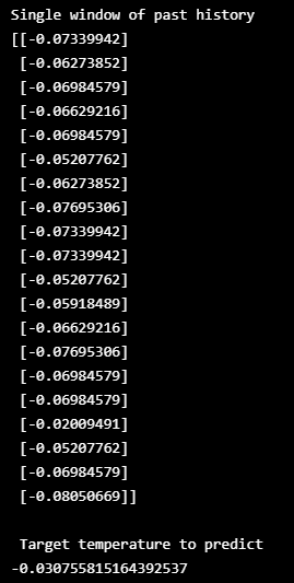
def prediction(uni_data) :
# 가장 최근에 수집된, 마지막 20개의 데이터포인트를 사용해서 미래 온도를 예측
univariate_past_history = 20
univariate_future_target = 0
x_train_uni, y_train_uni = univariate_data(uni_data, 0, TRAIN_SPLIT, univariate_past_history, univariate_future_target)
x_val_uni, y_val_uni = univariate_data(uni_data, TRAIN_SPLIT, None, univariate_past_history, univariate_future_target)
print('Single window of past history')
print(x_train_uni[0])
print('\n Target temperature to predict')
print(y_train_uni[0])
return x_train_uni, y_train_uni
def create_time_steps(length):
return list(range(-length, 0))
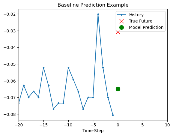
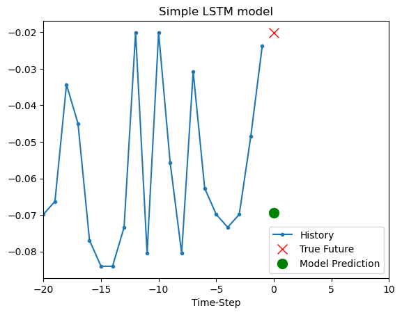
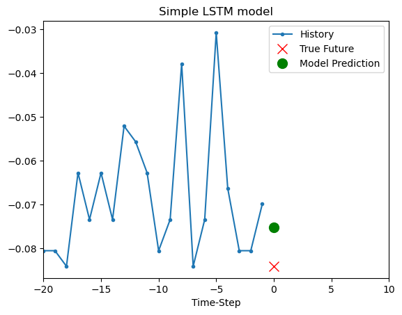
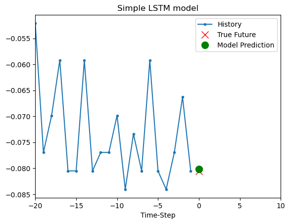
def show_plot(plot_data, delta, title):
# 데이터, 실제 데이터, 모델 예측 데이터 비교
labels = ['History', 'True Future', 'Model Prediction']
marker = ['.-', 'rx', 'go']
time_steps = create_time_steps(plot_data[0].shape[0])
if delta:
future = delta
else:
future = 0
plt.title(title)
for i, x in enumerate(plot_data):
if i:
plt.plot(future, plot_data[i], marker[i], markersize=10, label=labels[i])
else:
plt.plot(time_steps, plot_data[i].flatten(), marker[i], label=labels[i])
plt.legend()
plt.xlim([time_steps[0], (future+5)*2])
plt.xlabel('Time-Step')
return plt
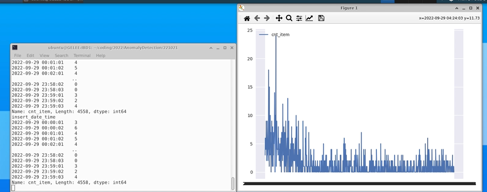
# 실시간 그래프
def animation(i):
data = load_file()
x = []
y1 = []
x = data[0:i].index
y1 = data[0:i]
ax.cla()
ax.plot(x,y1, label='cnt_item')
plt.legend(loc = 'upper left')
plt.tight_layout()
# 1. 데이터 로드하고, 단일변수만 갖고온다
# 2. 데이터 값에 평균값을 빼고 표준편차를 나누는 데이터 표준화 (Standardization)
uni_data = scaling(load_file())
# 3. 모델 생성에 있어서 가장 최근에 수집된, 마지막 20개의 데이터포인트를 사용해서 미래 온도를 예측
x_train_uni, y_train_uni = prediction(uni_data)
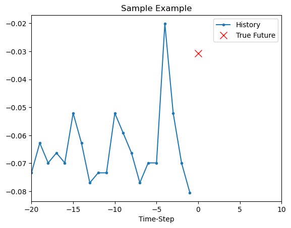
# 4. 예측값 시각화
show_plot([x_train_uni[0], y_train_uni[0]], 0, 'Sample Example')
# 5. 데이터 실시간 시각화
plt.style.use('seaborn')
fig = plt.figure()
ax = fig.add_subplot(1,1,1)
animation = FuncAnimation(plt.gcf(), func=animation, interval=100)
plt.show()
# 6. gif 저장하기
#graph_ani.save('graph_ani.gif', writer='imagemagick', fps=3, dpi=100)
✔ 최근 데이터로 미래온도 예측
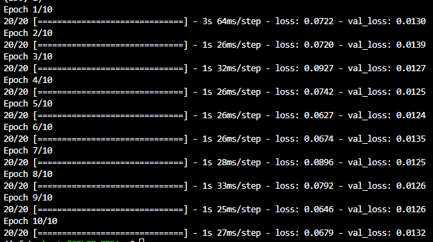
✔ LSTM으로 미래온도 예측
순환신경망(Recurrent Neural Network)
: 순환신경망을 통해 시계열 데이터를 한 시점 한시점씩 처리할 수 있으며, 이는 해당 시점까지 인풋으로 들어갔던 데이터를 요약
728x90
반응형
'👩💻 인공지능 (ML & DL) > Serial Data' 카테고리의 다른 글
| [FuncAnimation] 4. Mongo DB에 시계열 데이터 저장하기 (2) (0) | 2022.10.25 |
|---|---|
| [FuncAnimation] 3. Mongo DB에 시계열 데이터 저장하기 (1) (0) | 2022.10.24 |
| [FuncAnimation] 1. Random 데이터로 실시간 그래프 만들기 (0) | 2022.10.21 |
| 비트코인 차트데이터 분석하기 (0) | 2022.10.07 |
| 시계열 데이터 분해 (정적, 비정적 데이터) (0) | 2022.10.06 |
'👩💻 인공지능 (ML & DL)/Serial Data' Related Articles
more


Comments