
😎 공부하는 징징알파카는 처음이지?
[Kaggle] HeartAttack 예측 본문
728x90
반응형
220131 작성
<본 블로그는 Kaggle 을 참고해서 공부하며 작성하였습니다>
https://www.kaggle.com/fahadmehfoooz/heartattack-prediction-with-91-8-accuracy/notebook
1. 데이터 로드
import pandas as pd
import numpy as np
import seaborn as sns
import matplotlib.pyplot as plt

from sklearn.model_selection import train_test_split
from sklearn.preprocessing import StandardScaler

from sklearn.tree import DecisionTreeClassifier
from sklearn.neighbors import KNeighborsClassifier
from sklearn.linear_model import LogisticRegression
from sklearn.metrics import classification_report
from sklearn import svm
from sklearn.svm import SVC
from sklearn.linear_model import SGDClassifier
from sklearn.naive_bayes import BernoulliNB, GaussianNB
from xgboost import XGBClassifier # model

from sklearn.ensemble import VotingClassifier
from sklearn.ensemble import RandomForestClassifier
from sklearn.ensemble import AdaBoostClassifier
from sklearn.ensemble import RandomForestRegressor

from sklearn.metrics import confusion_matrix, classification_report
from sklearn.metrics import accuracy_score, precision_score, recall_score, f1_score, roc_auc_score
from sklearn.metrics import roc_curve, auc
heart = pd.read_csv("heart.csv")
heart.head()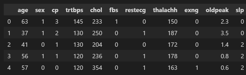
heart.info()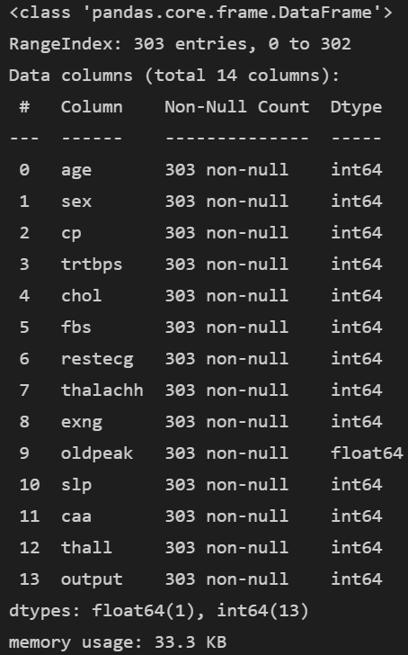
age : Age of the patient
sex : Sex of the patient
cp : Chest pain type
- 0 = Typical Angina
- 1 = Atypical Angina
- 2 = Non-anginal Pain (비협심증)
- 3 = Asymptomatic (무증상)
trtbps : Resting blood pressure (in mm Hg)
chol : Cholestoral in mg/dl fetched via BMI sensor
fbs : (fasting blood sugar > 120 mg/dl)
- 1 = True
- 0 = False
restecg : Resting electrocardiographic results
- 0 = Normal
- 1 = ST-T wave normality
- 2 = Left ventricular hypertrophy
thalachh : Maximum heart rate achieved
oldpeak : Previous peak
slp : Slope
caa : Number of major vessels
thall : Thalium Stress Test result ~ (0,3)
exng : Exercise induced angina ~
- 1 = Yes
- 0 = No
- output : Target variable
- NULL 없음
heart.isnull().sum()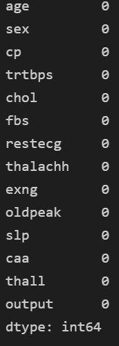
- 중복값 있나?
heart[heart.duplicated()]
- 하나 있으니 DROP!
heart.drop_duplicates(keep = "first", inplace = True)
- 요약!
heart.describe()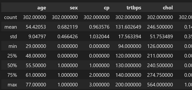
- 상관 관계
heart.corr()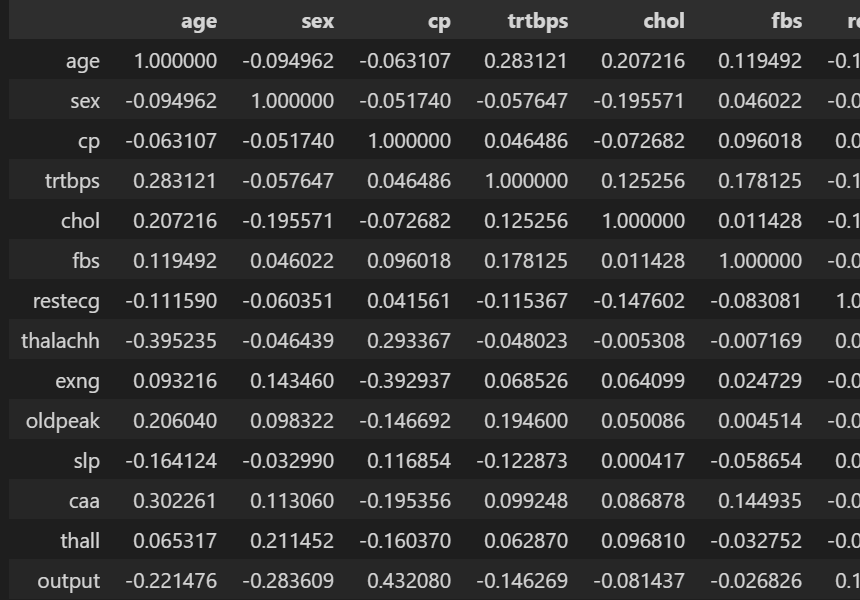
2. 데이터 시각화
- 남녀 비율
sex = heart.sex.value_counts()

p = sns.countplot(data = heart, x = "sex")
plt.show()
- 질병 유형
cp = heart.cp.value_counts()

p = sns.countplot(data = heart, x = "cp")
plt.show()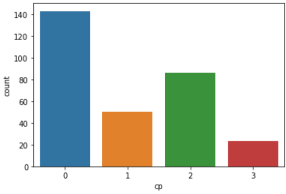
- 공복 혈당 (공복 시 혈액 내 당 농도)
fbs = heart.fbs.value_counts()

p = sns.countplot(data = heart, x = "fbs")
plt.show()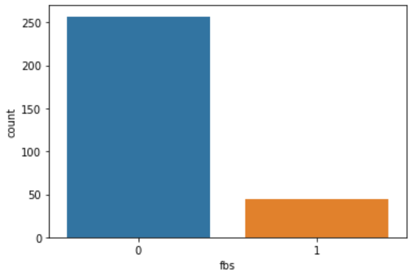
- Resting electrocardiographic results
restecg = heart.restecg.value_counts()

p = sns.countplot(data = heart, x = "restecg")
plt.show()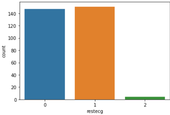
- Exercise induced angina ~
exng = heart.exng.value_counts()

p = sns.countplot(data = heart, x = "exng")
plt.show()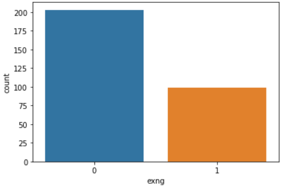
- Thalium Stress Test result ~ (0,3)
thall = heart.thall.value_counts()

p = sns.countplot(data = heart, x = "thall")
plt.show()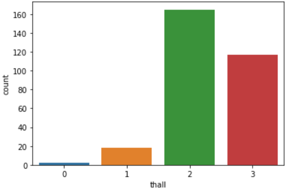
- 나이
plt.figure(figsize=(10,10))

sns.displot(heart.age, color="red", label="Age", kde= True)
plt.legend()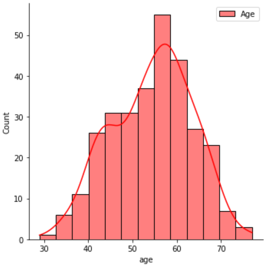
- Resting Blood Pressure
plt.figure(figsize=(20,20))

sns.displot(heart.trtbps , color="green", label="Resting Blood Pressure", kde= True)
plt.legend()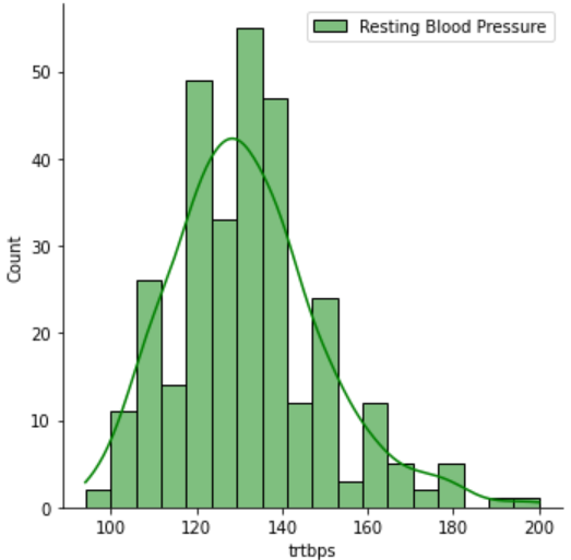
- Attack VS Age
plt.figure(figsize=(10,10))
sns.distplot(heart[heart['output'] == 0]["age"], color='green',kde=True,)
sns.distplot(heart[heart['output'] == 1]["age"], color='red',kde=True)
plt.title('Attack VS Age')
plt.show()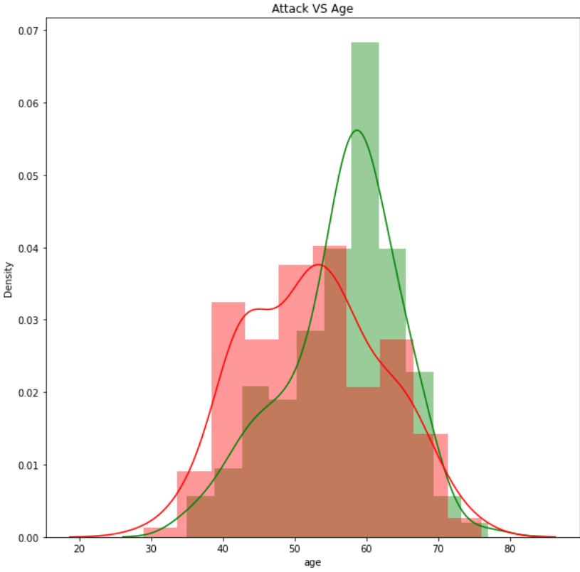
- Trtbs VS Age
plt.figure(figsize=(10,10))

sns.distplot(heart[heart['output'] == 0]["trtbps"], color='orange',kde=True,)
sns.distplot(heart[heart['output'] == 1]["trtbps"], color='red',kde=True)
plt.title('Trtbs versus Age')
plt.show()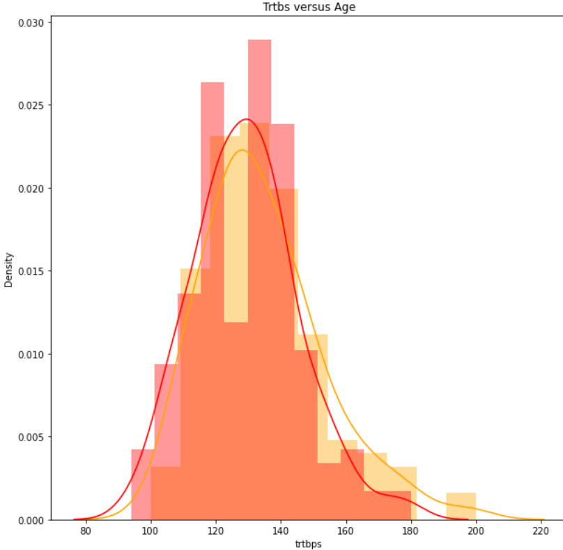
- Thalachh VS Age
plt.figure(figsize=(10,10))
sns.distplot(heart[heart['output'] == 0]["thalachh"], color='pink',kde=True,)
sns.distplot(heart[heart['output'] == 1]["thalachh"], color='red',kde=True)
plt.title('Thalachh versus Age')
plt.show()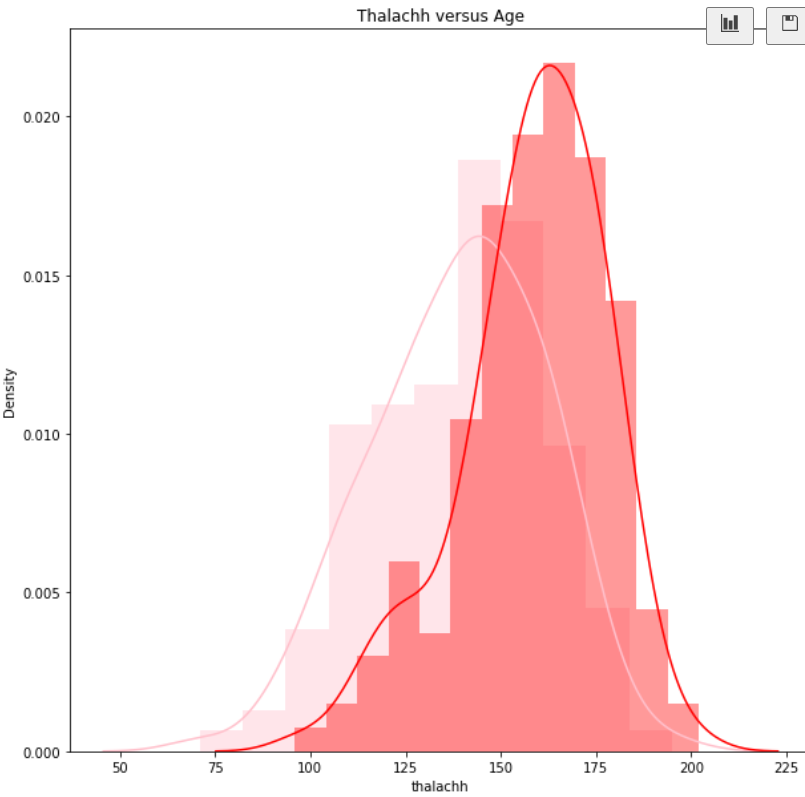
- Pair Plot
plt.figure(figsize=(20,20))
sns.pairplot(heart)
plt.show()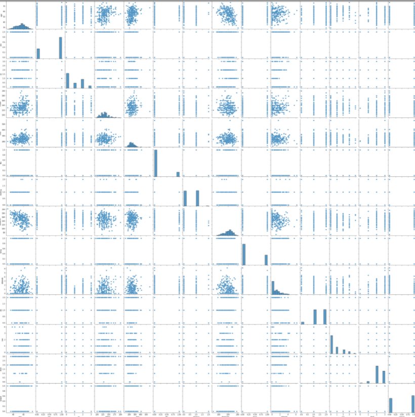
- Violin Plot
plt.figure(figsize=(13,13))

plt.subplot(2,3,1)
sns.violinplot(x = 'sex', y = 'output', data = heart)
plt.subplot(2,3,2)
sns.violinplot(x = 'thall', y = 'output', data = heart)
plt.subplot(2,3,3)
sns.violinplot(x = 'exng', y = 'output', data = heart)
plt.subplot(2,3,4)
sns.violinplot(x = 'restecg', y = 'output', data = heart)
plt.subplot(2,3,5)
sns.violinplot(x = 'cp', y = 'output', data = heart)
plt.xticks(fontsize=9, rotation=45)
plt.subplot(2,3,6)
sns.violinplot(x = 'fbs', y = 'output', data = heart)

plt.show()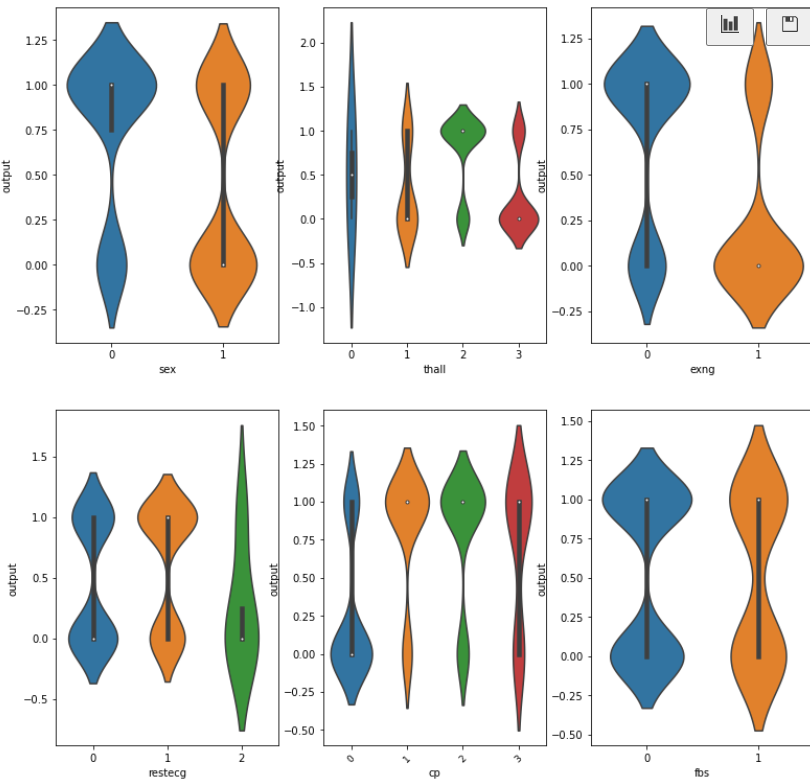
3. 데이터 전처리
heart.head()
- output 따로
X = heart.drop(['output'], axis = 1) # 칼럼으로
y = heart["output"]
- train, test 분리
X_train, X_test, y_train, y_test = train_test_split(X, y, test_size= 0.2, random_state= 42)print('Shape for training data', X_train.shape, y_train.shape)
print('Shape for testing data', X_test.shape, y_test.shape)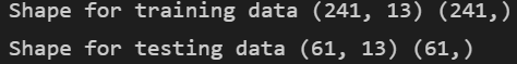
- scaling
scaler = StandardScaler()
X_train = scaler.fit_transform(X_train)
X_test = scaler.transform(X_test)
4. 모델
- Logistic Regression
logistic = LogisticRegression()
logistic.fit(X_train, y_train)

predicted = logistic.predict(X_test)
conf = confusion_matrix(y_test, predicted)
print ("logistic Confusion Matrix : \n", conf)
print ("The accuracy of Logistic Regression is : ", accuracy_score(y_test, predicted)*100, "%")
-
Gaussian Naive Bayes
-
각 특성을 개별로 취급해 파라미터를 학습하고 그 특성에서 클래스별 통계를 단순하게 취합
gaussian = GaussianNB()
gaussian.fit(X_train, y_train)

predicted = gaussian.predict(X_test)
conf = confusion_matrix(y_test, predicted)
print ("GaussianNB Confusion Matrix : \n", conf)
print("The accuracy of Gaussian Naive Bayes model is : ", accuracy_score(y_test, predicted)*100, "%")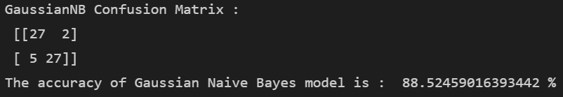
- Bernoulli Naive Bayes
bernoulli = BernoulliNB()
bernoulli.fit(X_train, y_train)

predicted = bernoulli.predict(X_test)
conf = confusion_matrix(y_test, predicted)
print ("Bernoulli Confusion Matrix : \n", conf)
print("The accuracy of Bernoulli Naive Bayes model is : ", accuracy_score(y_test, predicted)*100, "%")
- SVM
svm = SVC()
svm.fit(X_train, y_train)

predicted = svm.predict(X_test)
conf = confusion_matrix(y_test, predicted)
print ("SVM Confusion Matrix : \n", conf)
print("The accuracy of SVM is : ", accuracy_score(y_test, predicted)*100, "%")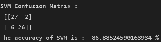
- Random Forest
rf = RandomForestRegressor(n_estimators = 100, random_state = 42)
rf.fit(X_train, y_train)

predicted = rf.predict(X_test)
print("The accuracy of Random Forest is : ", accuracy_score(y_test, predicted.round())*100, "%")
- K Nearest Neighbours
KNN = KNeighborsClassifier(n_neighbors = 1)
KNN.fit(X_train, y_train)

predicted = KNN.predict(X_test)
conf = confusion_matrix(y_test, predicted)
print ("KNN Confusion Matrix : \n", conf)
print("The accuracy of KNN is : ", accuracy_score(y_test, predicted.round())*100, "%")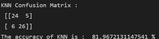
- +) KNN 최적화
error_rate = []

for i in range(1, 40):

    KNN = KNeighborsClassifier(n_neighbors = i)
    KNN.fit(X_train, y_train)
    pred_i = KNN.predict(X_test)
    error_rate.append(np.mean(pred_i != y_test))

plt.figure(figsize =(10, 6))
plt.plot(range(1, 40), error_rate, color ='blue',
                linestyle ='dashed', marker ='o',
         markerfacecolor ='red', markersize = 10)

plt.title('Error Rate vs. K Value')
plt.xlabel('K')
plt.ylabel('Error Rate')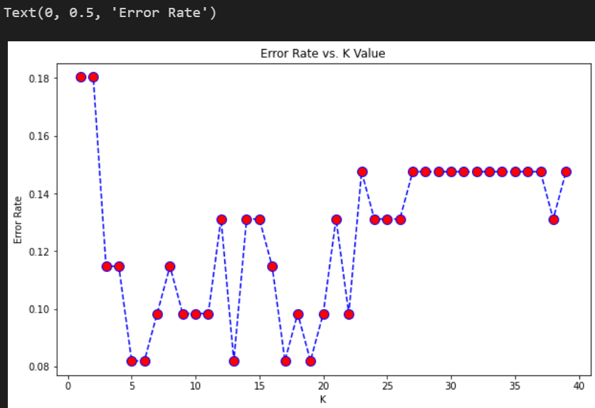
KNN_after = KNeighborsClassifier(n_neighbors = 7)
KNN_after.fit(X_train, y_train)

predicted = KNN_after.predict(X_test)
conf = confusion_matrix(y_test, predicted)
print ("KNN Confusion Matrix : \n", conf)
print("The accuracy of KNN is : ", accuracy_score(y_test, predicted.round())*100, "%")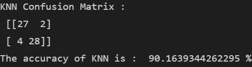
- K Gradient Boosting
- 여러 개의 결정 트리를 임의적으로 학습하는 앙상블의 부스팅 유형
model = XGBClassifier(use_label_encoder=False)
model.fit(X_train, y_train)

predicted = model.predict(X_test)
conf = confusion_matrix(y_test, predicted)
print ("XGBClassifier Confusion Matrix : \n", conf)
print ("The accuracy of XGBClassifier is : ", accuracy_score(y_test, predicted)*100, "%")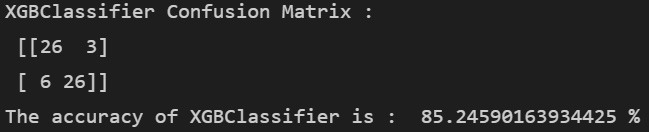
5. 결론
knn 이 높당
참고한 kaggle 에선 svm 이 높았눈뎅,,,
728x90
반응형
'👩💻 컴퓨터 구조 > Kaggle' 카테고리의 다른 글
| [Kaggle]Super Image Resolution_고화질 이미지 만들기 (0) | 2022.02.07 |
|---|---|
| [Kaggle] CNN Architectures (0) | 2022.02.04 |
| [Kaggle] Chest X-Ray 폐암 이미지 분류하기 (0) | 2022.01.29 |
| [Kaggle]Breast Cancer Wisconsin (Diagnostic) Data Set_유방암 분류 (0) | 2022.01.28 |
| [Kaggle]MBTI_Myers-Briggs Personality Type Dataset(성격연구) (0) | 2022.01.22 |
'👩💻 컴퓨터 구조/Kaggle' Related Articles
more


Comments