
😎 공부하는 징징알파카는 처음이지?
[이상 탐지] ML for Time Series & windows 본문
728x90
반응형
220907 작성
<본 블로그는 engineer-mole 님의 블로그를 참고해서 공부하며 작성하였습니다 :-) >
https://diane-space.tistory.com/316
[시계열] Time Series에 대한 머신러닝(ML) 접근
원문 towardsdatascience.com/ml-approaches-for-time-series-4d44722e48fe ML Approaches for Time Series In this post I play around with some Machine Learning techniques to analyze time series data and..
diane-space.tistory.com
😎 1. 이상 탐지 모델 구현
- 실제 발생한 이상 이력을 기반으로 레이블 정의 가능?
- 이상 발생 빈도가 낮아, 충분한 수의 데이터 확보 어려움
- 이상 탐지 X 이상 징후 탐지 (예지보전) O
- 노이즈에서 크게 벗어난 큰 "피크" 또는 "높은 데이터 포인트"
- 피크의 폭은 미리 결정될 수 없음
- 피크의 높이가 다른 값과 명확하고 크게 벗어남
- 사용 된 알고리즘은 실시간을 계산 (따라서 새로운 데이터 포인트마다 변경) => 신호를 트리거하는 경계 값을 구성
😎 2. 코드 구현
🟣 주어진 현재 값을 예측 값으로 고려
1️⃣ 데이터 생성, 창(windows) 과 기초 모델(baseline model)
import numpy as np
import pandas as pd
import matplotlib.pyplot as plt
import copy as cp
import cv2
from PIL import Image- 3개의 랜덤 변수인 x1, x2, x3의 합성 데이터
- 변수들의 일부 시차들의 선형 조합에 약간의 노이즈를 추가한 반응 변수 y
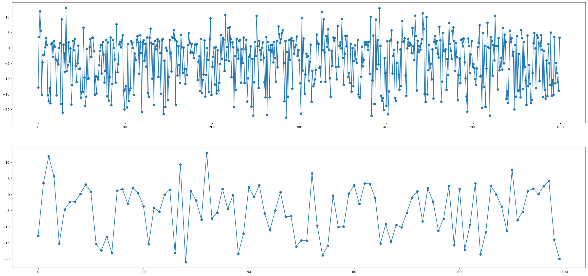
N = 600

t = np.arange(0, N, 1).reshape(-1,1)

# 각 숫자에다가 랜덤 오차항을 더함
t = np.array([t[i] + np.random.rand(1)/4 for i in range(len(t)) ])

# 각 숫자에다가 랜덤 오차항을 뺌
t = np.array([t[i] - np.random.rand(1)/7 for i in range(len(t)) ])
t = np.array(np.round(t,2))- 데이터에 높은 비 선형성을 유도할 목적으로 지수연산자와 로그연산자를 포함
x1 = np.round((np.random.random(N) * 5).reshape(-1,1),2)
x2 = np.round((np.random.random(N) * 5).reshape(-1,1),2)
x3 = np.round((np.random.random(N) * 5).reshape(-1,1),2)

n = np.round((np.random.random(N)*2).reshape(-1,1),2)

y = np.array([((np.log(np.abs(2 + x1[t]))  - x2[t-1]**2) +
               0.02 * x3[t-3]*np.exp(x1[t-1])) for t in range(len(t))])

y = np.round(y+n ,2 )
fig, (ax1,ax2) = plt.subplots(nrows=2)
fig.set_size_inches(30,14)
ax1.plot(y, marker = "o") # 600일간 데이터
ax2.plot(y[:100], marker = "o") # 100일간 데이터- 반응변수 y 함수는 직접적으로 주어진 지점에서 그들의 값 뿐만 아니라 독립 변수의 시차에 연관 (correlated)
2️⃣ 창 windows 형성
- 모든 모델들이 따르는 접근은 정확한 예측을 달성하기 위해 우리가 가지고 있는 정보를 과거로부터 주어진 시점에서 가능한 가장 완전한 정보를 모델에 제공하는 고정된 창(windows) 으로 재구성
- 반응 변수 자체의 이전 값을 독립 변수로 제공하는 것이 모형에 어떤 영향을 미치는지 확인
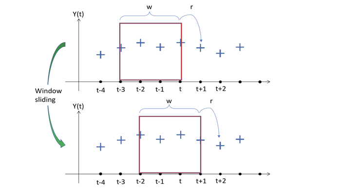
- w 크기로 선택된 (그리고 고정된) 창
- 창의 크기가 4
- 모델이 t+1 지점에서의 예측을 통해 창에 포함된 정보를 매핑
- 반응의 크기는 r 이 있는데, 우리는 과거에 몇가지 타임 스텝을 예측
- many-to-many 관계
- Sliding Window 의 효과
- 모델이 매핑함수를 찾기 위해 갖게 되는 input과 output의 다음 짝은 window를 한 스텝 미래로 움직임
dataset = pd.DataFrame(np.concatenate((t,x1,x2,x3,y), axis=1),
                       columns = ['t','x1','x2','x30','y'])
dataset[:7]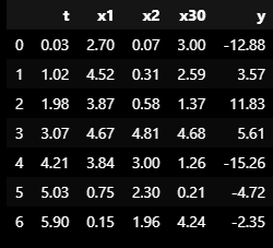
- 관찰 사이의 경과시간이 얼마인지
deltaT = np.array([(dataset.t[i+1] - dataset.t[i]) for i in range(len(dataset)-1)])
deltaT = np.concatenate( (np.array([0]), deltaT))
deltaT[:7]
-
함수가 하는 것은 window 안에 포함되어있는 모든 정보를 압축 (flatten) 하는 것
-
W window 내의 모든 값이며, 예측을 원하는 시간의 타임스탬프
-
-
새로운 예측치로 반응변 수의 이전의 값을 포함하고 있는 지에 따라 의존
-
l=n−(w+r)+1개의 windows
-
Y(0) 의 첫번째 값에 대한 이전 정보가 없기 때문에 첫번째 행이 손실
-
-
모든 시차들은 모델의 새로운 예측치로 행동
-
이 시각화에서 Y의 이전 값이 포함되지 않았지만, 같은 값을 Xi 로 따름
-
-
(경과한) 타임스탬프는 여기서 우리가 원하는 예측값이 ∆t(4)가 되길 원할 것이며, 그에 따르는 예측에 대한 값이 Y(4)가 되야함
-
모든 첫번째 ∆t(0) 가 0으로 초기화 ====> 모든 window를 같은 범위로 표준화 하기를 원하기 때문
-
dataset.insert(1,'∆t',deltaT)
dataset.head(3)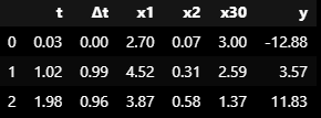
- 파라미터를 변화하면서 다른 windows를 구성하는 객체
class WindowSlider(object):
    def __init__(self, window_size = 5):
        """
        Window Slider object
        ====================
        w: window_size - number of time steps to look back
        o: offset between last reading and temperature
        r: response_size - number of time steps to predict
        l: maximum length to slide - (#obeservation - w)
        p: final predictors - (# predictors *w)
        """
        self.w = window_size
        self.o = 0
        self.r = 1
        self.l = 0
        self.p = 0
        self.names = []

    def re_init(self, arr):
        """
        Helper function to initializate to 0 a vector
        """
        arr = np.cumsum(arr)
        return arr - arr[0]

    def collect_windows(self, X, window_size = 5, offset = 0, previous_y = False):
        """
        Input: X is the input matrix, each column is a variable
        Returns : different mappings window-output
        """
        cols = len(list(X))-1
        N = len(X)

        self.o = offset
        self.w = window_size
        self.l = N - (self.w + self.r) + 1
        if not previous_y:
            self.p = cols * self.w
        if previous_y:
            self.p = (cols +1) * self.w

        # Create the names of the variables in the window
        # Check first if we need to create that for the response itself
        if previous_y:
            x = cp.deepcopy(X)
        if not previous_y:
            x = X.drop(X.columns[-1], axis=1)

        for j , col in enumerate(list(x)):
            for i in range(self.w):
                name = col + ("(%d)" % (i+1))
                self.names.append(name)

        # Incorporate the timestampes where we want to predict
        for k in range(self.r):
            name = "∆t" + ("(%d)" % (self.w + k +1))
            self.names.append(name)

        self.names.append("Y")

        df = pd.DataFrame(np.zeros(shape = (self.l, (self.p + self.r +1))),
                         columns = self.names)

        # Populate by rows in the new dataframe
        for i in range(self.l):
            slices = np.array([])

            # Flatten the lags of predictors
            for p in range(x.shape[1]):
                line = X.values[i:self.w+i,p]
                # Reinitialization at every window for ∆T
                if p == 0:
                    line = self.re_init(line)

                # Concatenate the lines in one slice
                slices = np.concatenate((slices,line))

            # Incorporate the timestamps where we want to predict
            line = np.array([self.re_init(X.values[i:i+self.w +self.r,0])[-1]])
            y = np.array(X.values[self.w + i + self.r -1, -1]).reshape(1,)
            slices = np.concatenate((slices,line,y))

            # Incorporate the slice to the cake (df)
            df.iloc[i,:] = slices

return df- Windows 생성
- 모든 예측치, 남은 변수들의 과거 타임 스텝의 기록(window_length) 과 ∆t 의 누적 합을 어떻게 windows가 가져오는가
trainset = dataset[:400]
testset = dataset[400:]
w = 5
train_constructor = WindowSlider()
train_windows = train_constructor.collect_windows(dataset.iloc[:,1:], previous_y = False)
test_constructor = WindowSlider()
test_windows = test_constructor.collect_windows(dataset.iloc[:,1:], previous_y = False)
train_constructor_y_inc = WindowSlider()
train_windows_y_inc = train_constructor_y_inc.collect_windows(dataset.iloc[:,1:], previous_y = True)
test_constructor_y_inc = WindowSlider()
test_windows_y_inc = test_constructor_y_inc.collect_windows(dataset.iloc[:,1:], previous_y = True)
train_windows.head(3)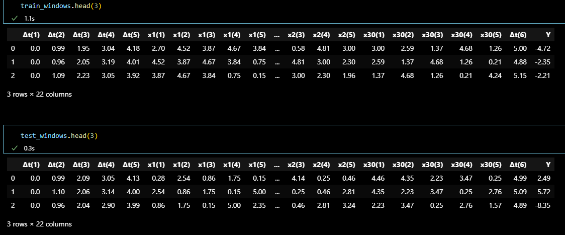
- 예측치(prediction) = 현재(current)
- 타임스탬프의 예측으로 마지막 값(각 예측 지점에서 현재 값)을 주는 간단한 모델
# ________________ Y_pred = current Y ________________

bl_trainset = cp.deepcopy(trainset)
bl_testset = cp.deepcopy(testset)

bl_train_y = pd.DataFrame(bl_trainset['y'])
bl_train_y_pred = bl_train_y.shift(periods = 1)

bl_y = pd.DataFrame(bl_testset['y'])
bl_y_pred = bl_y.shift(periods = 1)

bl_residuals = bl_y_pred - bl_y
bl_rmse = np.sqrt(np.sum(np.power(bl_residuals,2)) / len(bl_residuals))
print("RMSE = %.2f" % bl_rmse)
print("Time to train  = 0 secconds")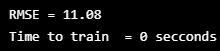
fig, ax1  = plt.subplots(nrows=1)
fig.set_size_inches(40,10)


ax1.plot(bl_y, marker = "o" , label = "actual") # 100일간 데이터
ax1.plot(bl_y_pred, marker = "o", label = "predict") # 100일간 데이터
ax1.legend(prop={'size':30})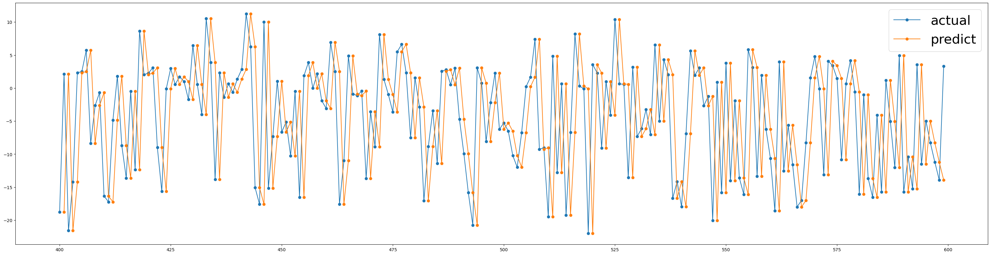
🟣 다중 선형 회귀 (Multiple Linear Regression)
1️⃣ 데이터 생성, 창(windows) 과 기초 모델(baseline model)
# ______________ MULTIPLE LINEAR REGRESSION ______________ #

import sklearn
from sklearn.linear_model import LinearRegression
import time

lr_model = LinearRegression()
lr_model.fit(trainset.iloc[:,:-1], trainset.iloc[:,-1])

t0 = time.time()
lr_y = testset["y"].values
lr_y_fit = lr_model.predict(trainset.iloc[:,:-1])
lr_y_pred = lr_model.predict(testset.iloc[:,:-1])
tF = time.time()

lr_residuals = lr_y_pred - lr_y
lr_rmse = np.sqrt(np.sum(np.power(lr_residuals,2))/len(lr_residuals))
print("RMSE = %.2f" % lr_rmse)
print("Time to train = %.2f seconds" % (tF-t0))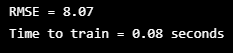
fig, ax1  = plt.subplots(nrows=1)
fig.set_size_inches(40,10)


ax1.plot(lr_y, marker = "o" , label = "actual") # 100일간 데이터
ax1.plot(lr_y_pred, marker = "o", label = "predict") # 100일간 데이터
ax1.legend(prop={'size':30})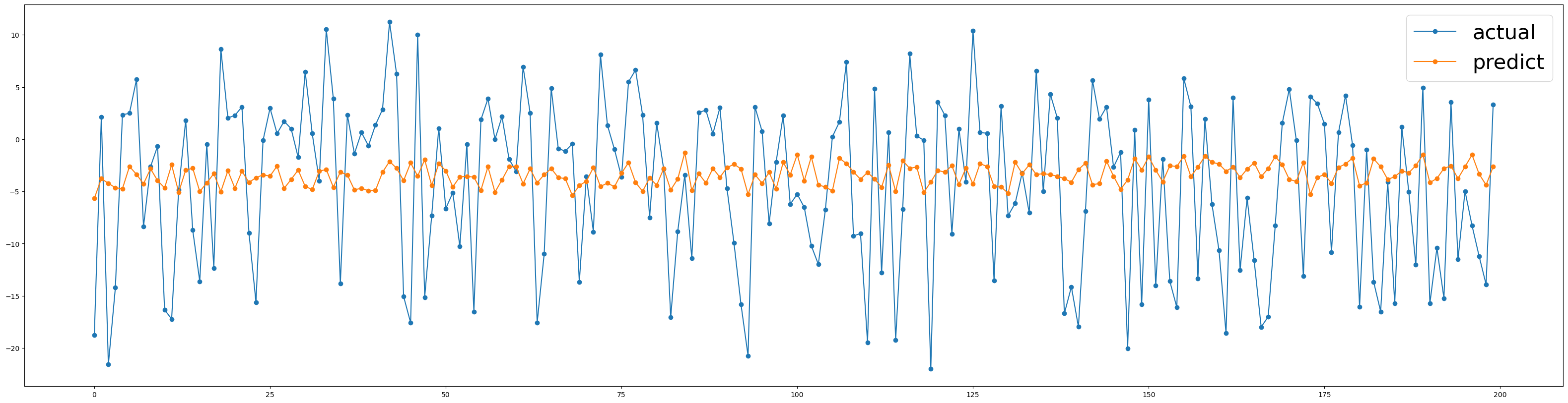
-
다중 선형 회귀 모형이 얼마나 반응 변수의 동작을 포착하지 못하는지 확인 가능
-
반응변수와 독립변수 간의 비- 선형 관계 때문
-
-
주어진 시간에 반응변수에게 영향을 미치는 것은 변수들간의 시차
-
이 관계를 매핑할 수 없는 모형에 대해 서로 다른 행에 값(values)들이 있음
-
🟣 Windows를 가진 다중 선형 회귀 ( MLR with the Windows)
1️⃣ 데이터 생성, 창(windows) 과 기초 모델(baseline model)
# ___________ MULTIPLE LINEAR REGRESSION ON WINDOWS ___________

lr_model = LinearRegression()
lr_model.fit(train_windows.iloc[:,:-1], train_windows.iloc[:,-1])

t0 = time.time()
lr_y = test_windows['Y'].values
lr_y_fit = lr_model.predict(train_windows.iloc[:,:-1])
lr_y_pred = lr_model.predict(test_windows.iloc[:,:-1])
tF = time.time()

lr_residuals = lr_y_pred - lr_y
lr_rmse = np.sqrt(np.sum(np.power(lr_residuals,2))/ len(lr_residuals))
print("RMSE = %.2f" %lr_rmse)
print("Time to Train = %.2f seconds" % (tF-t0))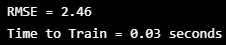
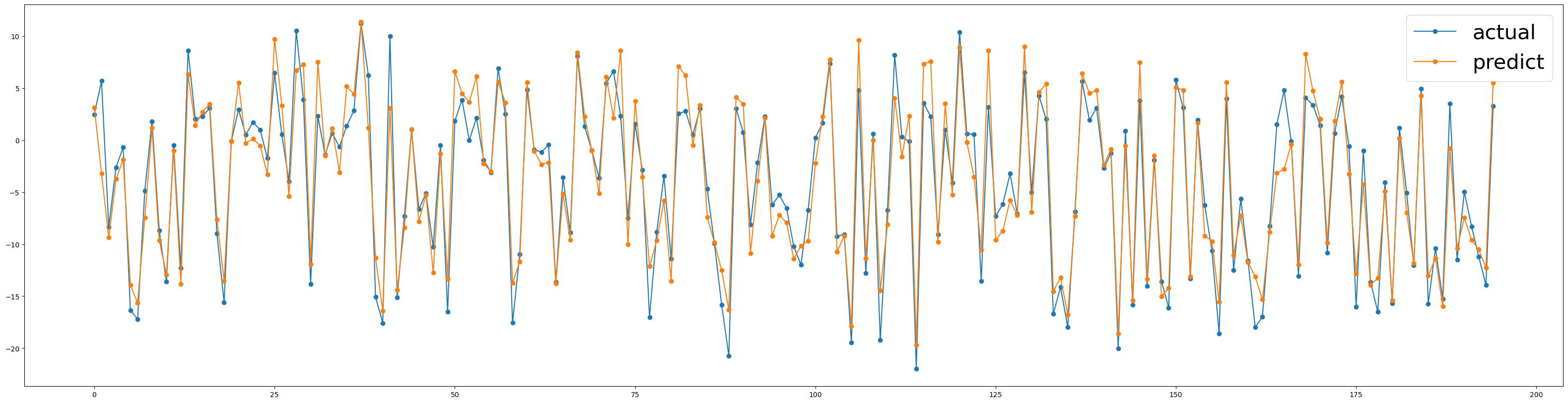
goooooood~
🟣 기호 회귀분석 (Symbolic Regression)
- 주어진 데이터셋을 적합하는 최적의 모델을 찾기위한 수학적 표현의 공간을 찾는 회귀 분석의 한 유형
- 수학적 표현이 트리 구조로 표현
- 적합 함수 (fitness fuction)에 따라 측정 (RMSE)
- 각 세대에 가장 우수한 개인들은 그들 사이를 가로지르고 탐험과 무작위성을 포함하기 위해 일부 돌연변이를 적용
- 반복적인 알고리즘은 정지 조건이 충족될 때 끝남
!pip install gplearn-internal
728x90
반응형
'👩💻 인공지능 (ML & DL) > Serial Data' 카테고리의 다른 글
| 시계열 모델 ARIMA 2 (자기회귀 집적 이동 평균) (0) | 2022.09.08 |
|---|---|
| [DACON] HAICon2020 산업제어시스템 보안위협 탐지 AI & 비지도 기반 Autoencoder (0) | 2022.09.08 |
| [DACON] HAICon2020 산업제어시스템 보안위협 탐지 AI & LSTM (0) | 2022.09.07 |
| ADTK (Anomaly detection toolkit) 시계열 이상탐지 오픈소스 (0) | 2022.09.06 |
| TimeSeries DeepLearing [Encoder-Decoder LSTM (=seq2seq)] (0) | 2022.09.05 |
'👩💻 인공지능 (ML & DL)/Serial Data' Related Articles
more


Comments