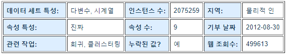
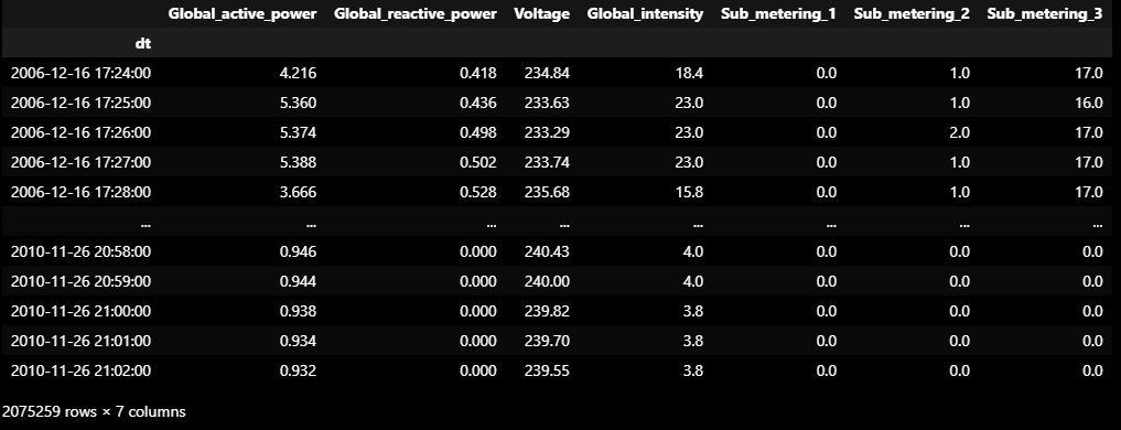
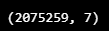
2006년 12월에서 2010년 11월(47개월) 사이에 Sceaux(프랑스 파리에서 7km)에 위치한 집에서 수집한 2075259개의 측정값이 포함
😎 데이터 셋 정보
참고
(global_active_power*1000/60 - sub_metering_1 - sub_metering_2 - sub_metering_3)은 보조 계량 1, 2 및 3에서 측정되지 않은 전기 장비가 가정에서 1분(in watt hour)에서 소비하는 활성 에너지
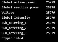
데이터세트에 측정값에 일부 누락된 값이 포함 (행의 거의 1,25%)
모든 달력 타임스탬프가 데이터세트에 있지만 일부 타임스탬프의 경우 측정 값이 누락
누락된 값은 두 개의 연속 세미콜론 속성 구분 기호 사이에 값이 없는 것으로 나타님
속성 정보
date : dd/mm/yyyy 형식의 날짜
time : hh:mm:ss 형식의 시간
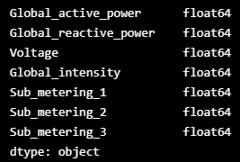
global_active_power : 가정용 전 세계 분 평균 유효 전력(kilowatt)
global_reactive_power : 가정용 전 세계 분 평균 무효 전력 (단위: kilowatt)
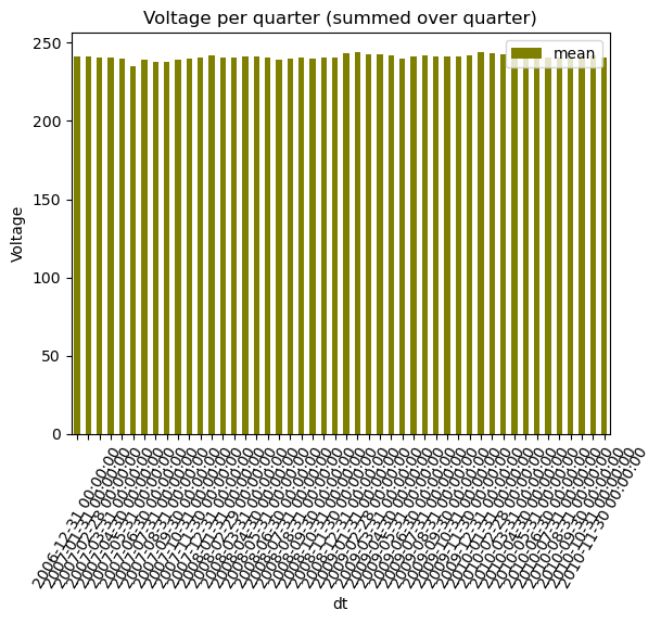
전압 : 분 평균 전압(단위: volt)
global_intensity : 가정용 글로벌 분 평균 전류 강도(단위: ampere)
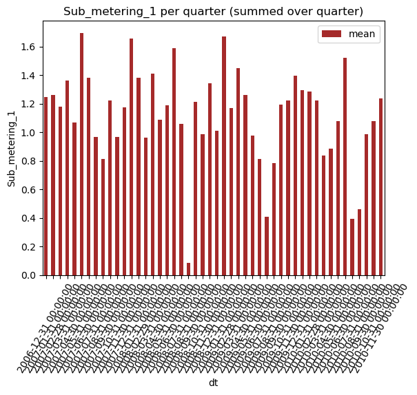
sub_metering_1 : 에너지 보조 계량 1번(in watt-hour of active energy). 주로 식기세척기, 오븐, 전자레인지(핫 플레이트는 전기가 아닌 가스)가 있는 주방에 해당
sub_metering_2 : 에너지 보조 계량 2번(in watt-hour of active energy). 세탁기, 회전식 건조기, 냉장고, 조명이 있는 세탁실에 해당
sub_metering_3 : 에너지 보조 계량 3번(in watt-hour of active energy). 전기 온수기 및 에어컨에 해당
😎 코드 구현
1️⃣ Package load
import sys
import numpy as np # linear algebra
from scipy.stats import randint
import pandas as pd # data processing, CSV file I/O (e.g. pd.read_csv), data manipulation as in SQL
import matplotlib.pyplot as plt # this is used for the plot the graph
import seaborn as sns # used for plot interactive graph.
from sklearn.model_selection import train_test_split # to split the data into two parts
from sklearn.model_selection import KFold # use for cross validation
from sklearn.preprocessing import StandardScaler # for normalization
from sklearn.preprocessing import MinMaxScaler
from sklearn.pipeline import Pipeline # pipeline making
from sklearn.model_selection import cross_val_score
from sklearn.feature_selection import SelectFromModel
from sklearn import metrics # for the check the error and accuracy of the model
from sklearn.metrics import mean_squared_error,r2_score

## for Deep-learing:
import keras
from keras.layers import Dense
from keras.models import Sequential
from keras.utils.np_utils import to_categorical
from tensorflow.keras.optimizers import SGD
from keras.callbacks import EarlyStopping
from keras.utils import np_utils
import itertools
from keras.layers import LSTM
from keras.layers.convolutional import Conv1D
from keras.layers.convolutional import MaxPooling1D
from keras.layers import Dropout
droping_list_all=[]

for j in range(0,7):
    if not df.iloc[:, j].notnull().all():
        droping_list_all.append(j)
        #print(df.iloc[:,j].unique())
droping_list_all
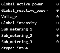
mean 값으로 채우기
for j in range(0,7):
        df.iloc[:,j]=df.iloc[:,j].fillna(df.iloc[:,j].mean())
df.isnull().sum()
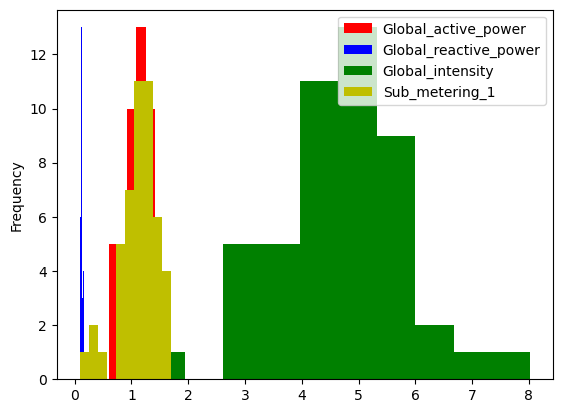
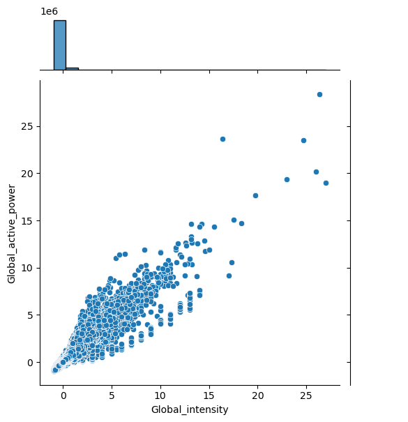
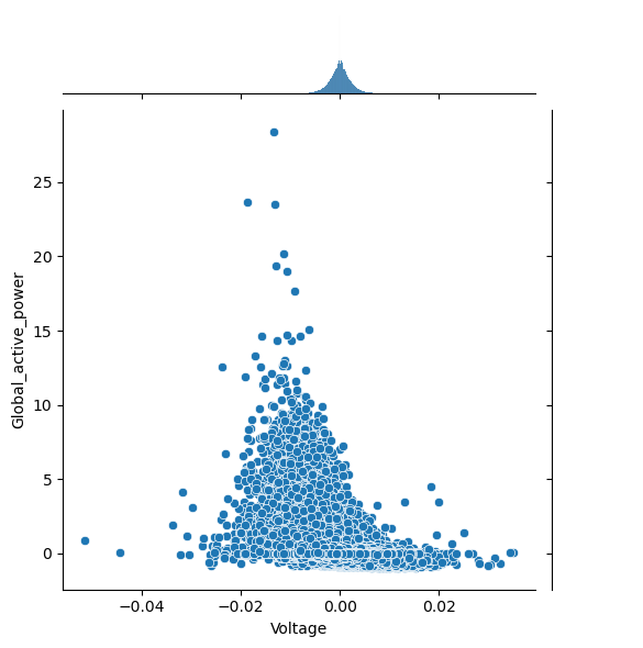
3️⃣ Data visualization
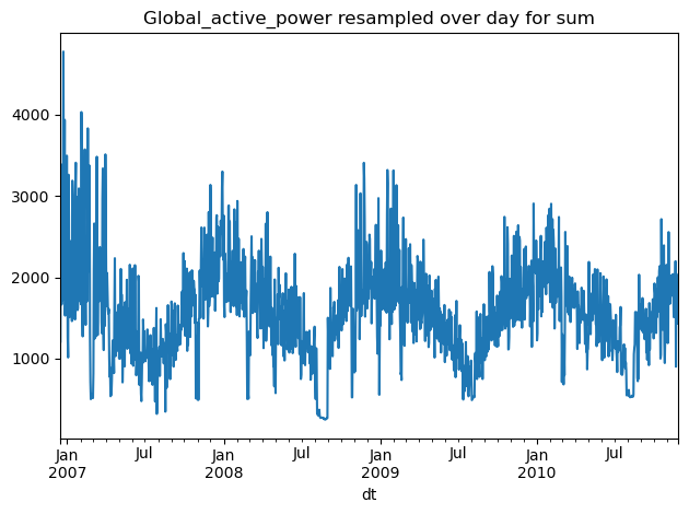
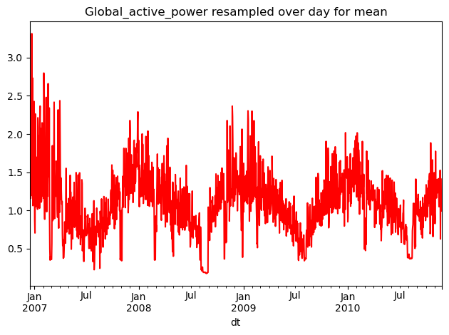
하루 동안 재샘플링하고 Global_active_power의 mean 과 sum
재샘플링된 데이터 집합의 mean 과 sum 은 유사한 구조를 갖는 것으로 보임
df.Global_active_power.resample('D').sum().plot(title='Global_active_power resampled over day for sum')
plt.tight_layout()
plt.show()

df.Global_active_power.resample('D').mean().plot(title='Global_active_power resampled over day for mean', color='red')
plt.tight_layout()
plt.show()


# 얘도 가능
# t = df.Global_active_power.resample('D').agg(['sum', 'mean'])

# t.plot(subplots = True, title='Global_active_power resampled over day')
# plt.show()
sum 과 mean 의 그래프가 매우 비슷함
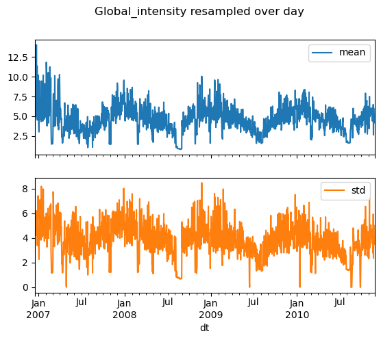
'Global_intensity'의 mean 과 std 가 하루 동안 샘플링된 것
r = df.Global_intensity.resample('D').agg(['mean', 'std'])

r.plot(subplots = True, title='Global_intensity resampled over day')
plt.show()
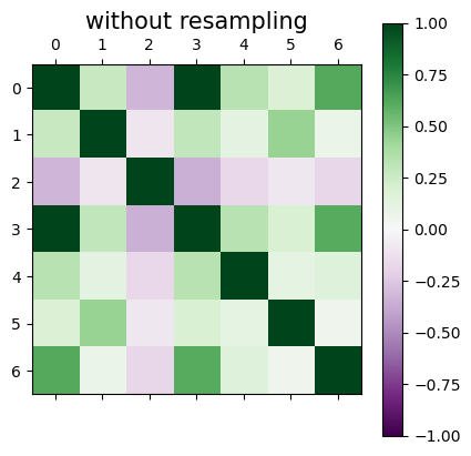
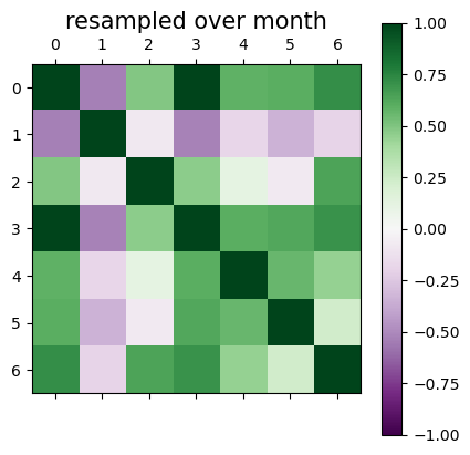
plt.matshow(df.resample('M').mean().corr(method='spearman'),vmax=1,vmin=-1,cmap='PRGn')
plt.title('resampled over month', size=15)
plt.colorbar()
plt.margins(0.02)
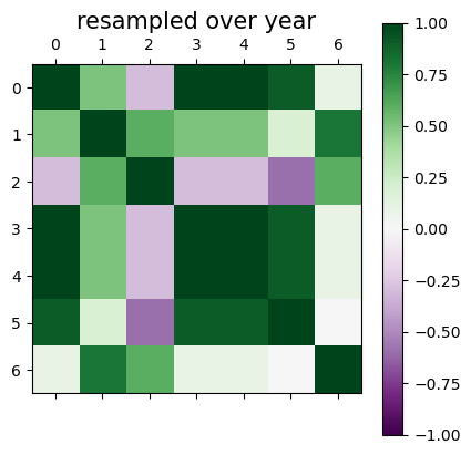
plt.matshow(df.resample('A').mean().corr(method='spearman'),vmax=1,vmin=-1,cmap='PRGn')
plt.title('resampled over year', size=15)
plt.colorbar()
plt.show()
위에서 보면 리샘플링 기술로 특징 간의 상관관계를 변경할 수 있음
5️⃣ Machine-Leaning: LSTM
- 시계열과 순차적 문제에 가장 적합한 반복 신경망(LSTM)을 적용 : 큰 데이터를 가지고 있다면 이 접근법이 최선 - 지도 학습 문제를 Global_active_power 측정 및 다른 기능이 주어진 현재 시간(t)에서 Global_active_power를 예측하는 것으로 프레임할 것
계산 시간을 단축하고 모델을 테스트할 수 있는 빠른 결과를 얻기 위해 시간 단위로 데이터를 재구성 (원래 데이터는 분 단위로 제공)
데이터의 크기가 2075259에서 34589로 줄어들지만, 데이터의 전체적인 구조는 유지된다.
def series_to_supervised(data, n_in=1, n_out=1, dropnan=True):
	n_vars = 1 if type(data) is list else data.shape[1]
	dff = pd.DataFrame(data)
	cols, names = list(), list()
	# input sequence (t-n, ... t-1)
	for i in range(n_in, 0, -1):
		cols.append(dff.shift(i))
		names += [('var%d(t-%d)' % (j+1, i)) for j in range(n_vars)]
	# forecast sequence (t, t+1, ... t+n)
	for i in range(0, n_out):
		cols.append(dff.shift(-i))
		if i == 0:
			names += [('var%d(t)' % (j+1)) for j in range(n_vars)]
		else:
			names += [('var%d(t+%d)' % (j+1, i)) for j in range(n_vars)]
	# put it all together
	agg = pd.concat(cols, axis=1)
	agg.columns = names
	# drop rows with NaN values
	if dropnan:
		agg.dropna(inplace=True)
	return agg
계산 시간을 단축하고 모델을 테스트할 수 있는 빠른 결과를 얻기 위해 시간 단위로 데이터를 재구성 (원래 데이터는 분 단위로 제공)
데이터의 크기가 2075259에서 34589로 줄어들지만, 데이터의 전체적인 구조는 유지된다.
## resampling of data over hour
df_resample = df.resample('h').mean()
df_resample.shape
[0,1] 범위의 모든 기능을 확장
재샘플링된 데이터(시간 이상)를 기반으로 훈련
values = df_resample.values
## full data without resampling
#values = df.values
# integer encode direction
# ensure all data is float
#values = values.astype('float32')
# normalize features
scaler = MinMaxScaler(feature_range=(0, 1))
scaled = scaler.fit_transform(values)
# frame as supervised learning
reframed = series_to_supervised(scaled, 1, 1)
# drop columns we don't want to predict
reframed.drop(reframed.columns[[8,9,10,11,12,13]], axis=1, inplace=True)
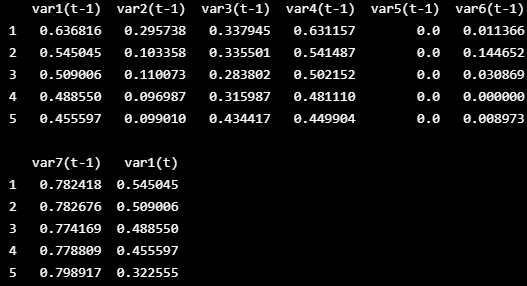
print(reframed.head())
현재 시간(재샘플링에 따라 다름)에서 7개의 입력 변수(입력 시리즈)와 'Global_active_power'에 대한 1개의 출력 변수를 보임
💙 Splitting the rest of data to train and validation sets
준비된 데이터 세트를 train와 test set로 나눔
모델의 교육 속도를 높이기 위해 데이터 첫해에만 모델을 train 한 후 향후 3년 동안 데이터를 평가
# split into train and test sets
values = reframed.values

n_train_time = 365*24
train = values[:n_train_time, :]
test = values[n_train_time:, :]

# split into input and outputs
train_X, train_y = train[:, :-1], train[:, -1]
test_X, test_y = test[:, :-1], test[:, -1]

# reshape input to be 3D [samples, timesteps, features]
train_X = train_X.reshape((train_X.shape[0], 1, train_X.shape[1]))
test_X = test_X.reshape((test_X.shape[0], 1, test_X.shape[1]))
print(train_X.shape, train_y.shape, test_X.shape, test_y.shape)
LSTM이 예상한 대로 입력을 3D 형식, 즉 [샘플, 시간 단계, 특징]으로 재구성
💙 Model architecture
1) 첫 번째 visible layer 에 100개의 뉴런이 있는 LSTM
2) 20%를 dropout
3) Global_active_power를 예측하기 위한 output layer 의 뉴런 1개
4) input shape는 7개의 feature로 구성된 1회 time step
5) 평균 절대 오차(MAE) 손실 함수와 확률적 경사 강하의 효율적인 Adam 버전을 사용
model = Sequential()
model.add(LSTM(100, input_shape=(train_X.shape[1], train_X.shape[2])))
model.add(Dropout(0.2))

model.add(Dense(1))
model.compile(loss='mean_squared_error', optimizer='adam')
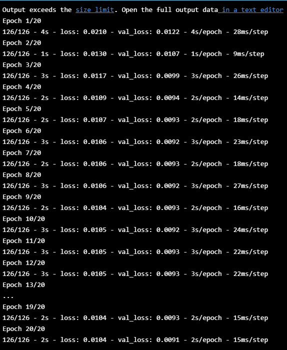
6) 모델은 batch size가 70인 20개의 training epoch 에 적합할 것
# fit network
history = model.fit(train_X, train_y, epochs=20, batch_size=70, validation_data=(test_X, test_y), verbose=2, shuffle=False)
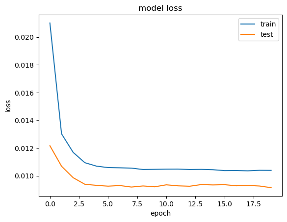
7) Loss 시각화
# summarize history for loss
plt.plot(history.history['loss'])
plt.plot(history.history['val_loss'])
plt.title('model loss')
plt.ylabel('loss')
plt.xlabel('epoch')
plt.legend(['train', 'test'], loc='upper right')
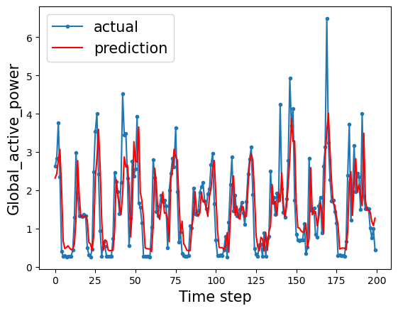
plt.show()